
The International Sociological Association 19th World Congress of Sociology in Toronto (15-21 July) has received quite some Twitter coverage. Waiting to board the flight back to Warsaw, I wanted to take a look at these Twitter data and apply the newly acquired skills in text analysis (thanks to the Summer Institute for Computational Social Science, SICSS, Partner Site in Tvärminne and Helsinki, Finland).
A few years ago my colleagues from the Polish Academy of Sciences and I wrote a paper about the inequality in national representation at ISA events (congresses and fora) 1. Analyses in this post reveals a different type of inequality at ISA conferences.
Getting data from Twitter
Tweets are an increasingly popular source of data for social scientists, not least because they can be quickly and conveniently obtained through the Twitter API. There are many excellent tutorials about how to connect to Twitter to download tweets, e.g. on the SICSS website.
First, the necessary packages:
#devtools::install_github("mkearney/rtweet") # newest version of rtweet from GitHub
library(rtweet) # for getting tweets from Twitter API
library(tidyverse) # data manipulation and cleaning
library(wordcloud) # for making world clouds
library(ggplot2) # for plotting
library(tidytext) # for tokenizing
library(lubridate) # dealing with dates
I downloaded tweets that contained one of the conference hashtags: #isa2018wcs or #isa18wcs (the hashtag is just like any other string to filter tweets). Twitter downloads typically contain tweets from the last ~10 days, and the set of tweets can change from download to download. This is why I saved the downloaded tweets in a .csv file for future use. The code for downloading and saving tweets with the ISA 2018 World Congress of Sociology was as follows:
isa <- search_tweets("#isa2018wcs OR #isa18wcs", since = "2018-06-01", n = 100000, type="recent", include_rts=TRUE)
data.table::fwrite(isa, file = "isa_tweets.csv")
isa <- read.csv("data/isa-twitter.csv", stringsAsFactors = FALSE) # open Twitter extract
isa$status_id <- as.character(isa$status_id)
isa$created_at <- as.POSIXct(strptime(isa$created_at, format = "%Y-%m-%dT%H:%M:%S")) # convert string to date and time
isa$created_at <-  with_tz(isa$created_at, 'America/New_York') # set time zone
I requested tweets starting with June 1, 2018, but this is unrealistic given Twitter’s restrictions, so I will check what’s the earliest tweet date. It’s July 12 morning.
min(isa$created_at)## [1] "2018-07-12 07:43:02 EDT"In total the data contain 9401 tweets (including 6478 retweets), around 1500-1700 on Congress days, and much fewer before and after the conference.
isa %>% group_by(day(created_at)) %>% count() # count tweets separately for each day## # A tibble: 11 x 2
## # Groups: day(created_at) [11]
## `day(created_at)` n
## <int> <int>
## 1 12 36
## 2 13 109
## 3 14 129
## 4 15 490
## 5 16 1672
## 6 17 1558
## 7 18 1789
## 8 19 1681
## 9 20 1374
## 10 21 510
## 11 22 53And here are the texts of a few sample tweets:
head(isa$text)## [1] "We're proud to publish Shirley Anne Tate's #book series Critical Mixed Race Studies (first title in the series, Remi Joseph-Salisbury's \"Black Mixed-Race Men\" out next month). Learn more about the series here: https://t.co/VbuXyDHJg5 or at stand 40 at #isa2018wcs #RC05 @RemiJS90 https://t.co/iOBAivJB2W"
## [2] "The fabulous @AlaSirriyeh with her wonderful new book âThe Politics of Compassionâ @policypress #booktour #isa18wcs https://t.co/Cto3bXF20Q"
## [3] "We're proud to publish Shirley Anne Tate's #book series Critical Mixed Race Studies (first title in the series, Remi Joseph-Salisbury's \"Black Mixed-Race Men\" out next month). Learn more about the series here: https://t.co/VbuXyDHJg5 or at stand 40 at #isa2018wcs #RC05 @RemiJS90 https://t.co/iOBAivJB2W"
## [4] "Thanks David Tabara for convening excellent conversation re. environmental solutions at #isa2018wcs . Thanks for invite to give a pop-up presentation on Sustainable Canada Dialogues @DialogSustainab . Info on this solution-focused network: https://t.co/liWma5eJu5"
## [5] "Brilliant performance by the Red Urban Project to help close #isa2018wcs https://t.co/hFpuiJqwsM"
## [6] "#Selfie time as #isa2018wcs comes to an end in #Toronto @isarc24 #YYZ @DrAmandaSlevin @HaluzaDeLay @StewartDLockie https://t.co/DswifxJt37"Tweets over time
I want to see the volume of ISA 2018 WCS tweets changed over time: first for the whole period covered by the data extract and on the busiest day - July 18th.
ts_plot(isa, "1 hour") +
  labs(x = NULL, y = NULL,
    title = "Frequency of #isa2018wcs OR #isa18wcs tweets since July 12, 2018",
    subtitle = "Twitter counts by hour",
    caption = "Source: Data collected from Twitter's API via rtweet")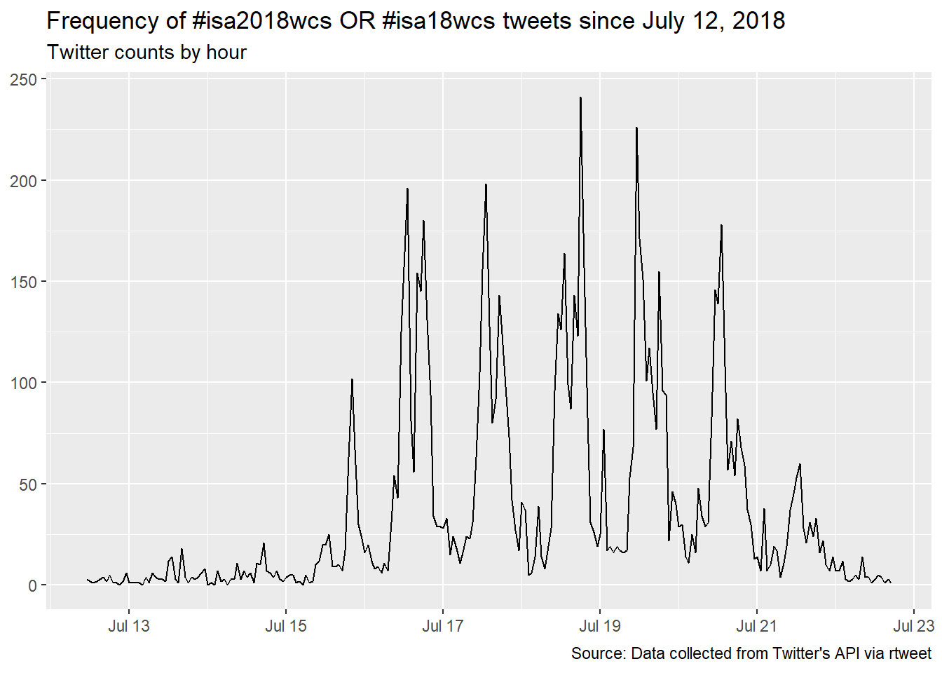
isa %>% filter(as.Date(created_at) >= "2018-07-18" & as.Date(created_at) < "2018-07-19") %>%
  ts_plot(., "5 minutes") +
    labs(x = NULL, y = NULL,
       title = "Frequency of #isa2018wcs OR #isa18wcs tweets on July 18, 2018",
       subtitle = "Twitter counts by 5 minutes",
       caption = "Source: Data collected from Twitter's API via rtweet")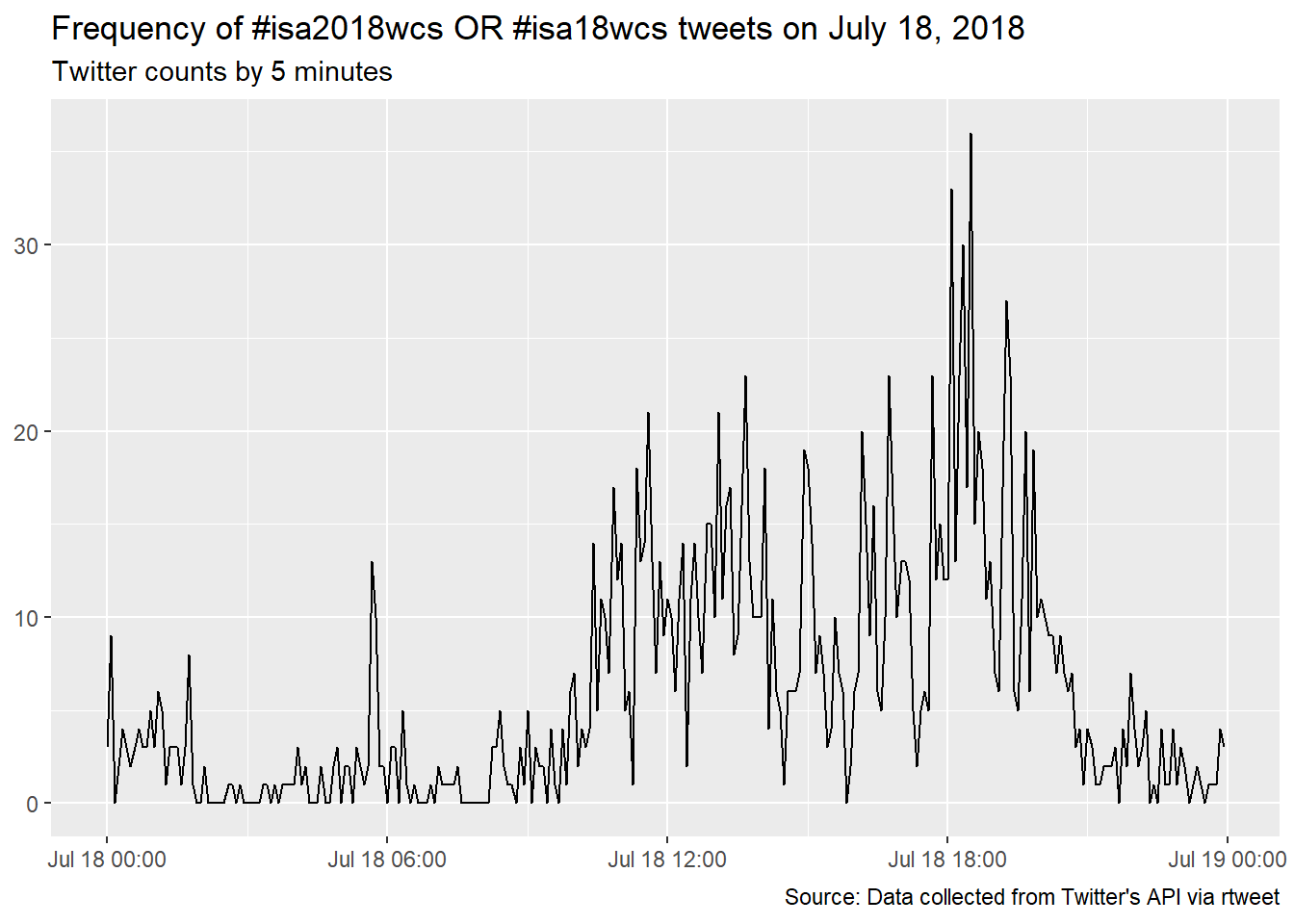
Overall it looks like the presentations around noon (11.30am - 1.20pm) and in the afternoon (3.30-5.20pm) were most tweet-provoking. Time stamps include hours, minutes and seconds, so it’s possible to link tweets to concrete sessions, if one is interested.
Text analysis
Before the tweets can be analyzed, they need to be tokenized (each word needs to become a separate record = row), and cleaned (stop words and other unnecessary strings need to be eliminated).
data("stop_words")

isa_words <- isa %>%
  unnest_tokens(word, text) %>%  # tokenize
  select(status_id, created_at, word) %>%  # select variables
  anti_join(stop_words) %>% # eliminate stop words  # remove stop words
  filter(!grepl("https|t.co|amp|rt|de|â|isa18wcs|isa2018wcs|isa_sociology|sociology|isa|session|toronto|canada|congress|conference",
              word)) %>% # remove unnecessary strings or obvious words
  filter(!grepl("\\b\\d+\\b", word)) # remove numbers
Here is the list of 10 most popular words. Perhaps not very surprising.
isa_words %>%
  count(word) %>%  # count word frequencies
  arrange(desc(n))  # sort by word frequency in a descending order
## # A tibble: 11,264 x 2
## word n
## <chr> <int>
## 1 social 936
## 2 research 742
## 3 violence 666
## 4 world 506
## 5 people 473
## 6 religion 455
## 7 australia 394
## 8 japan 378
## 9 africa 366
## 10 paper 366
## # ... with 11,254 more rowsTweets by ISA Resesarch Committee
Research committees (RC) are the core organizational unit in ISA. Research Committees bring together scholars interested in the same topic, e.g. political sociology or sociology of education. Right now there are 57 RCs.
I noticed that many tweets have RC hashtags, so I wanted to see which RC got the most tweets and how equal or unequal the distribution of tweets was. To do this, I count the number of times each RC is mentioned in the collected tweets. I’m assuming that all string patterns rc[digit][digit] refer to a research commitee (some RCs have single-digit numbers, but they are commonly referred to as “RC-O-[digit]”). I’m also assuming that RCs have no other hashtags than with the mentioned string pattern.
isa_rc <- isa_words %>% filter(str_detect(tolower(word), "rc[0-9]{2}"))
isa_rc$rc <- str_extract(isa_rc$word, "rc[0-9]{2}")
head(isa_rc, 10)
## status_id created_at word rc
## 1 1.02111e+18 2018-07-22 13:01:17 rc05 rc05
## 2 1.0211e+18 2018-07-22 12:22:30 rc05 rc05
## 3 1.01899e+18 2018-07-16 16:49:29 rc24 rc24
## 4 1.01814e+18 2018-07-14 08:28:39 rc28 rc28
## 5 1.01904e+18 2018-07-16 20:17:07 rc28 rc28
## 6 1.02007e+18 2018-07-19 16:06:12 rc22 rc22
## 7 1.01968e+18 2018-07-18 14:34:17 rc32 rc32
## 8 1.01968e+18 2018-07-18 14:34:17 rc25 rc25
## 9 1.02033e+18 2018-07-20 09:34:58 rc22 rc22
## 10 1.02005e+18 2018-07-19 14:44:42 rc22 rc22Most tweets mention just one research committee, but some refer to two or more, particularly in the case of joint sessions. Some tweets also refer to the same RC with more than one hashtag, e.g. #rc34youth and #rc34toronto. These instances need to be collapsed to count as one.
isa_rc <- isa_rc %>% group_by(status_id, created_at, rc) %>% summarise(count = n())A simple word cloud reveals the unanimous winner in the RC tweet competition: RC34 Sociology of Youth.
wordcloud(isa_rc$rc, min.freq=1, random.color = TRUE, colors= palette(rainbow(20)))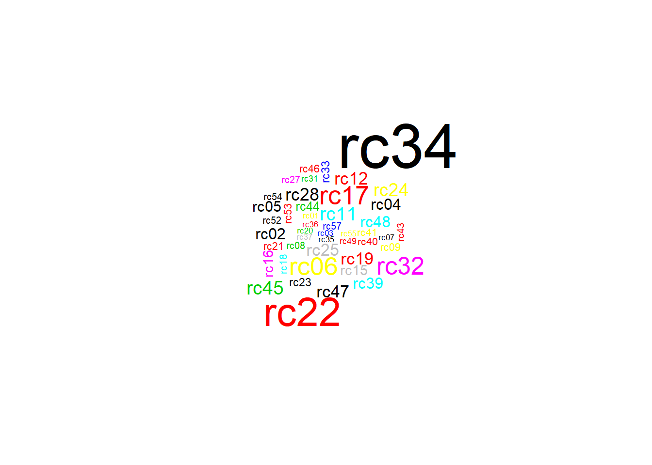
ggplot(isa_rc, aes(rc, fill = rc)) + geom_bar() +
  theme(axis.text.x = element_text(angle = 90, hjust = 2, vjust = 0.5), legend.position="none") +
  ylab("Number of tweets by Research Committee") +
  xlab("") +
  ggtitle("Tweets by Research Committee") +
  labs(caption = "Source: Data collected from Twitter's API via rtweet")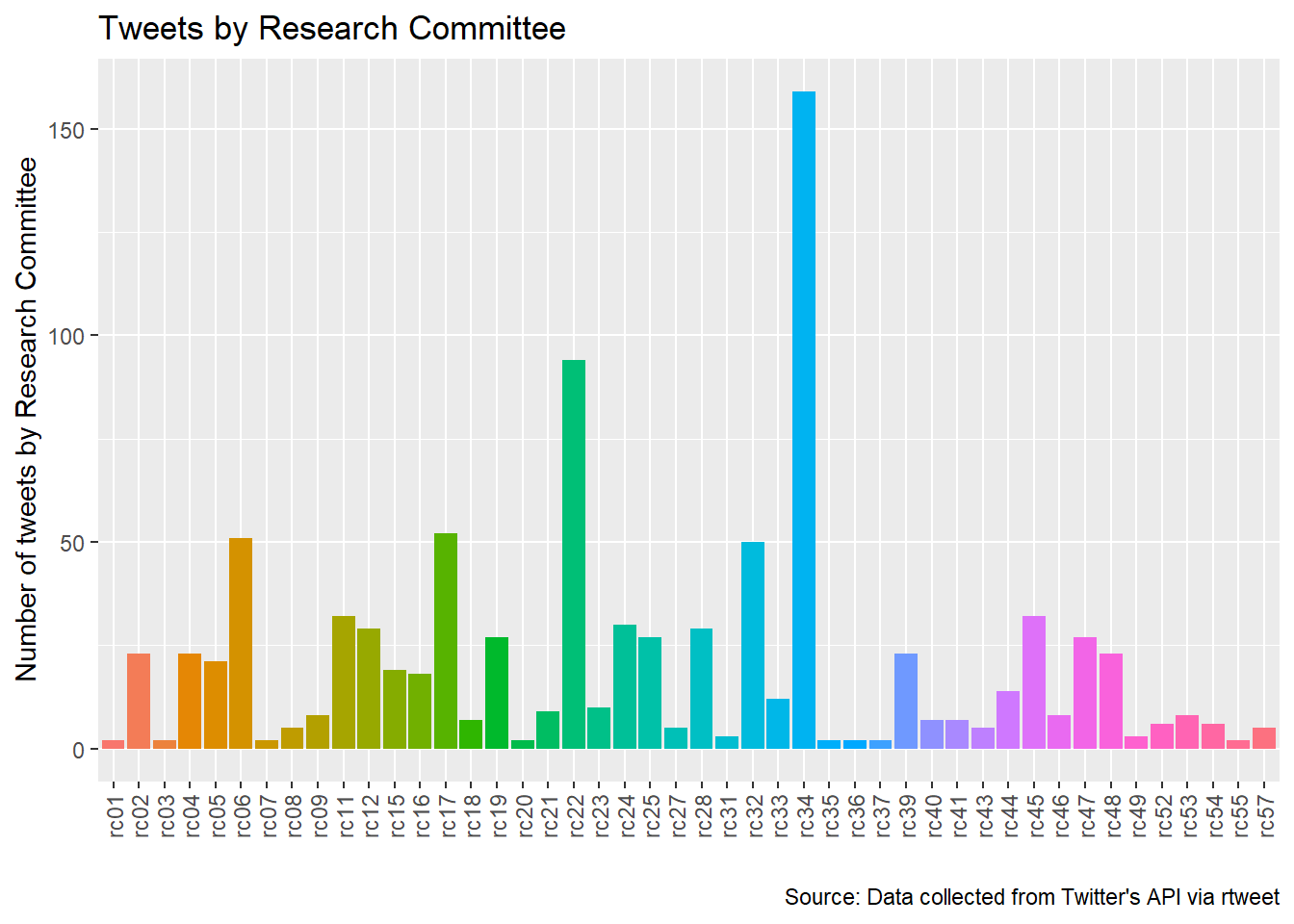
The bar plot confirms this result: RC34 is mentioned in the highest number of tweets and there is quite some variation in the number of tweets across RCs. If there is variation, maybe it can be explained. Some candidates: number of members, age of members, something about the leadership, area of specialization, quality of sessions, number of electrical outlets in the room?