Meritocracy is a principle according to which rewards are based on merit, as well as an ideal situation resulting from the operation of this principle. In their 1985 Social Foces paper titled “How Far to Meritocracy? Empirical Tests of a Controversial Thesis”, Tadeusz Krauze and Kazimierz M. Słomczyński proposed an algorithm to construct a theoretical joint distribution of education and income, given their marginal distributions, that would satisfy the conditions of meritocratic allocation. The meritocratic principle is simple: “more educated persons should not have lower social status than less educated ones”, which is equivalent to saying that “persons at a given level of education should have status levels equal to or higher than those of persons at a lower level of education” (Krauze and Slomczynski 1985: 628). Meritocracy is defined as the extent to which the observed distribution of income by education corresponds to the theoretical distribution under meritocracy. The difference between the observed and the meritocratic distribution is the distance to meritocracy.
In this post I show how to calculate the distance to meritocracy with simple R loops, using survey data on the example of the International Social Survey Project (ISSP) wave 2014. The code can be found here.
Determining meritocratic allocation
Cell proportions in the meritocratic allocation matrix (\(d_{i,j}\)) can be determined using the given marginals. The formula for the cell frequency \(d_{i,j}\), is as follows:
\[d_{i,j} = min(a_i — \sum_{k=0}^{j-1} d_{i,k}; b_i — \sum_{k=0}^{i-1} d_{k,j})\]
where \(i= 1,2,...,m\); \(j =1,2,...,n\), with \(m\) equal to the number of rows and \(n\) to the number of columns; \(a_i\) and \(b_j\) are margins of the observed distribution, and the terms \(d_{i,k}\) and \(d_{k,j}\) refer to the already determined entries of the meritocratic matrix (Krauze and Slomczynski 1985: 628).
How this works in practice is best illustrated with an example. The table below shows marginal distributions of education (highest completed education level) and personal income (5 categories; “Income 5” is the highest income category and “Income 1” is the lowest) in ISSP/2014 in Poland.
| Income 5 | Income 4 | Income 3 | Income 2 | Income 1 | ||
|---|---|---|---|---|---|---|
| Upper tertiary | 0.13811 | |||||
| Lower tertiary | 0.05299 | |||||
| Post-sec, non-tert. | 0.05588 | |||||
| Upper secondary | 0.55461 | |||||
| Lower secondary | 0.04645 | |||||
| Primary | 0.14386 | |||||
| No education | 0.00809 | |||||
| 0.24585 | 0.22634 | 0.16102 | 0.17557 | 0.19121 | 1.00000 |
The procedure starts from the cell corresponding to highest education and highest status, which is filled with the maximum possible proportion of people given the margins. This value is \(min(0.13811, 0.24585) = 0.13811\). Next, the remaining part of the “Income 5” margin \(0.24585 - 0.13811 = 0.10774\) is moved to the next highest education category (Lower tertiary). It doesn’t fit there, because the margin is 0.05299, so the remaining part of “Income 5” ends up in “Post-secondary non-tertiary”. After the cell “Post-secondary non-tertiary” and “Income 5” is filled and the margin form “Income 5” is exhausted, the remaining part of the “Post-secondary non-tertiary” margin is moved to “Income 4”. And the zig-zag continues until the whole table is filled out.
For the Polish ISSP/2014 sample, meritocratic allocation of income categories by education looks as follows:
| Income 5 | Income 4 | Income 3 | Income 2 | Income 1 | ||
|---|---|---|---|---|---|---|
| Upper tertiary | 0.13811 | 0.00000 | 0.00000 | 0.00000 | 0.00000 | 0.13811 |
| Lower tertiary | 0.05299 | 0.00000 | 0.00000 | 0.00000 | 0.00000 | 0.05299 |
| Post-sec, non-tert. | 0.05475 | 0.00113 | 0.00000 | 0.00000 | 0.00000 | 0.05588 |
| Upper secondary | 0.00000 | 0.22521 | 0.16102 | 0.16838 | 0.00000 | 0.55461 |
| Lower secondary | 0.00000 | 0.00000 | 0.00000 | 0.00719 | 0.03926 | 0.04645 |
| Primary | 0.00000 | 0.00000 | 0.00000 | 0.00000 | 0.14386 | 0.14386 |
| No education | 0.00000 | 0.00000 | 0.00000 | 0.00000 | 0.00809 | 0.00809 |
| 0.24585 | 0.22634 | 0.16102 | 0.17557 | 0.19121 | 1.00000 |
Meanwhile the empirical distribution looks like this:
| Income 5 | Income 4 | Income 3 | Income 2 | Income 1 | ||
|---|---|---|---|---|---|---|
| Upper tertiary | 0.08212 | 0.01689 | 0.01181 | 0.01512 | 0.01216 | 0.13811 |
| Lower tertiary | 0.02265 | 0.01104 | 0.00530 | 0.00680 | 0.00720 | 0.05299 |
| Post-sec, non-tert. | 0.01620 | 0.01669 | 0.00342 | 0.00699 | 0.01258 | 0.05588 |
| Upper secondary | 0.12048 | 0.15203 | 0.09404 | 0.08242 | 0.10563 | 0.55461 |
| Lower secondary | 0.00178 | 0.00718 | 0.01097 | 0.01717 | 0.00936 | 0.04645 |
| Primary | 0.00242 | 0.02206 | 0.03353 | 0.04312 | 0.04272 | 0.14386 |
| No education | 0.00020 | 0.00046 | 0.00194 | 0.00395 | 0.00155 | 0.00811 |
| 0.24585 | 0.22634 | 0.16102 | 0.17557 | 0.19121 | 1.00000 |
The difference between the empirical and the meritocratic distribution is as shown below, with positive values in green indicating cells where the empirical frequency is higher than the theoretical one, and negative values in blue indicating cells where the empirical frequency is lower than the theoretical frequency.
| Education | Income 5 | Income 4 | Income 3 | Income 2 | Income 1 |
|---|---|---|---|---|---|
| Upper tertiary | -0.05599 | 0.01689 | 0.01181 | 0.01512 | 0.01216 |
| Lower tertiary | -0.03034 | 0.01104 | 0.0053 | 0.0068 | 0.0072 |
| Post-sec, non-tert. | -0.03855 | 0.01556 | 0.00342 | 0.00699 | 0.01258 |
| Upper secondary | 0.12048 | -0.07318 | -0.06698 | -0.08596 | 0.10563 |
| Lower secondary | 0.00178 | 0.00718 | 0.01097 | 0.00998 | -0.0299 |
| Primary | 0.00242 | 0.02206 | 0.03353 | 0.04312 | -0.10114 |
| No education | 2e-04 | 0.00046 | 0.00194 | 0.00395 | -0.00654 |
Calculating the distance to meritocracy
The distance between the two bivariate distributions, one with the meritocratic allocation and the other with the empirical distribution, can be measured in various ways. One possible measure is the Earth Mover’s Distance (EMD), which represents the minimal effort required to turn one distribution into the other, taking into account the amount to be moved and the distance. In this way EMD is different from the Dissimilarity Index used originally by Krauze and Slomczynski (1985), as the latter is used for nominal variables and does not take into account the distance (number of ranks up or down) by which parts of the distribution need to be moved to match the meritocratic distribution.
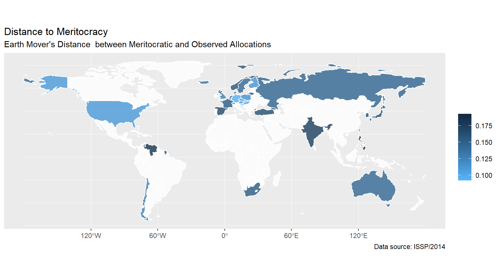
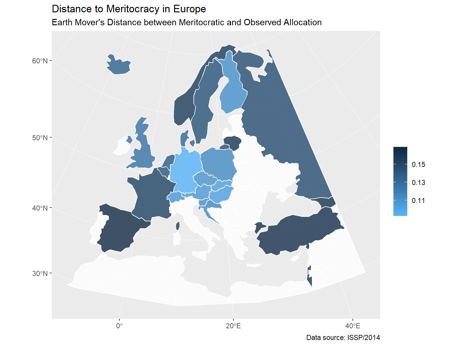
Distance to meritocracy by country
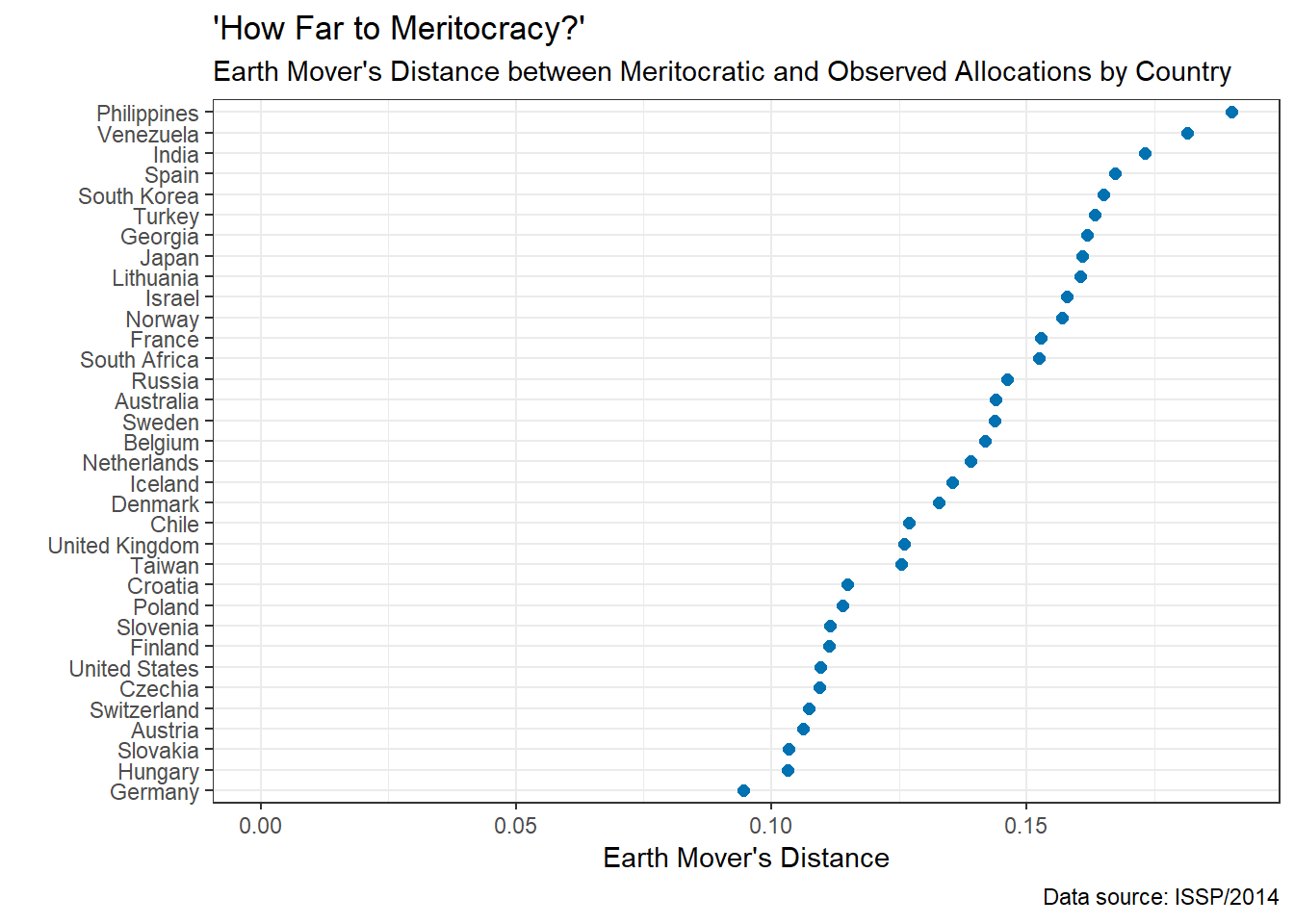
I identified the meritocratic distribution of income by education for countries included in ISSP/2014 using the procedure described earlier, and calculated the Earth Mover’s Distance between the country’s empirical and theoretical distributions. Manhattan distance is used in calculating the distances between cells of the table. The distance between two adjacent cells across rows (columns) was set to 1 / number of rows (columns).
The results are as shown on the dot plot below. Of the countries covered by ISSP/2014, Central Europe and the United States seem to be the most meritocratic, and the Philippines and Venezuela - the least meritocratic.
The world and Europe map visualize how distances to meritocracy are distributed geographically.