Downloading country-level indicators on participation and economic inequality

Data

We use the following datasets:

1. Varieties of Democracy (V-Dem)
   
2. Polyarchy
   
3. Freedom House
   
4. Polity IV
   
5. Democracy Barometer
   
6. The Standardized World Income Inequality Database (SWIID)
   
7. World Bank’s World Development Indicators

It is worth noting that there exists a package for downloading democracy indicators (democracyData), but it does not include the sub-indicators or sub-scales that are used to create the final composite scores, only the composite scores themselves. Still, it would be sufficient as a data source for many analyses.

Downloading data is the first step towards a combined dataset. To merge the indicators, it is also necessary to standardize country codes and year formats. The countrycode package is invaluable to convert between country code types. Years typically only need conversions between string and numeric types.

Packages

#devtools::install_github("xmarquez/vdem")
library(vdem) # gets V-Dem data
library(WDI) # gets data from World Bank's WDI
library(countrycode) # converts country codes
library(tidyverse) # for manipulating data
library(readxl) # for reading xls and xlsx files
library(haven) # for reading SPSS files
library(data.table) # fwrite to quickly write to CSV
library(ggplot2) # ggraphs

# custom color palette
myPalette <- c("#999999", "#E69F00", "#56B4E9", "#009E73", 
               "#F0E442", "#0072B2", "#D55E00", "#CC79A7")

Varieties of Democracy (V-Dem): Dedicated package

Varieties of Democracy (V-Dem) data can be downloaded via a dedicated R package (vdem), and a particular indicator can be selected with the parameter name_pattern.

The variable vdem_country_text_id already contains ISO3 character country codes (ISO3c), which is our preferred country code format.

vdem.part <- extract_vdem(name_pattern = "v2x_partipdem", include_uncertainty = FALSE) %>%
  select(iso3 = vdem_country_text_id, year, vdem_par = v2x_partipdem)

Polyarchy: Semicolon delimited CSV file

Polyarchy data are available as semicolon-delimited CSV files, as well as in Stata, SPSS, and Excel formats. The CSV format is the simplest, so this is the one we prefer. The read.csv2 function reads semicolon-delimited files as a default. Alternatively, read.csv could be used with an appropriate setting of the separator character.

Country codes are available in the Correlates of War format, which needs converting to ISO3c with the countrycode function. The year and the participation variables we are primarily interested in also need converting to numeric.

polyarchy <- read.csv2("https://www.prio.org/Global/upload/CSCW/Data/Governance/file42534_polyarchy_v2.csv",
                       stringsAsFactors = FALSE) %>%
  mutate(iso3 = countrycode(Abbr, "cowc", "iso3c")) %>%
  select(iso3, year = Year, polyarch_part = Part) %>%
  mutate(year = as.numeric(year),
         polyarch_part = as.numeric(polyarch_part))

Freedom House: Excel file with by-year sheets

Freedom House ratings started in 1973 but the subcategory scores are only available since 2006. They can be downloaded in an XLSX file with separate sheets including data for single years. The first sheet contains information about the contents of the remaining sheets, and the consecutive sheets contain information by year starting from the most recent year (2018), while the last sheet contains category scores (which are no use to us, since we need sub-category scores).

We encoutered problems trying to read in the file directly from the URL into R with the read.xlsx function, so we found a workaround where we download the file to a temporary folder and then open and manipulate it from there. It takes a moment to run but it works.

From the downloaded file we only need selected columns from selected sheets. To identify those sheets and columns, we first read all sheet names from the XLSX file and identify the sheets that contain the data we want to extract - those are sheets number 2 through 14.

Next we read all column names from one of the sheets with the data we are interested in (assuming that all remaining sheets have the same structure) - columns 1 (with country/territory names) and 6 (with the participation scores).

We loop through the sheets and store the extracted columns in a list. Then we append all elements of the list to create a country-year-level file.

Finally, we convert country/territory names to ISO3 codes and fix the issue of Kosovo, which does not have an official ISO3 code but the temporary one is “XKX”.

myurl <- "https://freedomhouse.org/sites/default/files/Aggregate%20Category%20and%20Subcategory%20Scores%20FIW2003-2018.xlsx" # sets URL to the file to be downloaded
td = tempdir() # reads in the path to the temp directory
tmp <- tempfile(tmpdir = td, fileext = ".xlsx") # creates path to the temp file in the temp directory
download.file(url = myurl, destfile = tmp, mode="wb") # downloads file from URL to the temp file with set extention
excel_sheets(tmp) # reads sheet names from the downloaded file
names(read_excel(path = tmp, sheet = 2)) # reads column names from the second sheet

fh.list <- list() # creates empty list to store selected parts of the 13 sheets
for (i in 1:13) {
  fh.list[[i]] <- read_excel(path = tmp, 
                             sheet = i+1) %>% # indexes (numbers) of columns to be extracted
    select(`Country/Territory`, fh_B_aggr = `B Aggr`) %>%
    mutate(country = gsub("[*].*$", "", `Country/Territory`),
           year = 2018 - i + 1) # adds year column
}

fh <- do.call("rbind", fh.list) %>% # binds (append) rows of all elements of fh.list
  mutate(iso3 = countrycode(country, "country.name", "iso3c")) %>%
  mutate(iso3 = ifelse(country %in% c("Kosovo", "Kosovo*"), "XKX", iso3)) %>%
  select(-country)

Polity IV: SPSS file

Polity IV distributes data in XLS and SAV (SPSS) formats. We had the same problems with directly reading the XLS file from the URL as with Freedom House, so we decided to use the SAV file instead. The only additional step we had to make beyond country code translations and setting the year variable ot numeric format was recoding of special codes in the polcomp variable (-66, -77, -88) to missing.

These special codes indicate foreign “interruptions” (-66), cases of “interregnum” or anarchy (-77), and “transition” (-88). For more information consult the Polity IV manual.

polity <- read_sav("http://www.systemicpeace.org/inscr/p4v2017.sav") %>%
  mutate(iso3 = countrycode(country, "country.name", "iso3c")) %>%
  mutate(iso3 = ifelse(country == "Kosovo", "XKX", iso3)) %>%
  select(iso3, year, p4_polcomp = polcomp) %>%
  mutate(p4_polcomp = ifelse(p4_polcomp %in% c(-66, -77, -88), NA, p4_polcomp))

Democracy Barometer: Excel file with header in top rows

The Democracy Barometer published its data in XLS, XLSX, and DTA (Stata) files. The DTA file curiously has only missing values on the variable of interest to us, so we use the XLS file. Like with Freedom House data, we download the file to a temporary folder and open from there. One modification that’s necessary is skipping the first four rows of the Excel sheet, which contain a header that needs to be removed prior to reading the data.

myurl <- "http://www.democracybarometer.org/Data/DB_data_1990-2016_Standardized.xls"
td = tempdir()
tmp <- tempfile(tmpdir = td, fileext = ".xls")
download.file(url = myurl, destfile = tmp, mode="wb")
excel_sheets(tmp)

db <- read_excel(tmp, skip = 4) %>%
  mutate(iso3 = countrycode(`Ccode QOG`, "iso3n", "iso3c")) %>%
  select(iso3, year = Year, db_PARTICIP = PARTICIP) %>%
  mutate(db_PARTICIP = as.numeric(db_PARTICIP))

The Standardized World Income Inequality Database (SWIID): Plain CSV file

Data from the Standardized World Income Inequality Database (SWIID) can be downloaded as a C file from Github.

swiid <- read.csv("https://raw.githubusercontent.com/fsolt/swiid/master/data/swiid7_1_summary.csv",
                  stringsAsFactors = FALSE, encoding = "UTF-8") %>%
  mutate(iso3 = countrycode(country, "country.name", "iso3c")) %>%
  mutate(iso3 = ifelse(country == "Kosovo", "XKX", iso3)) %>%
  select(iso3, year, gini_disp)

World Bank’s World Development Indicators: Dedicated package

Data from the World Bank’s World Development Indicators have a dedicated package WDI, which enables searching for data that contain a string (function WDIsearch) and downloading data for a selected indicator, country coverage and time range (WDI).

poverty <- WDI(country="all", indicator=c("SI.POV.NAHC"),
    start=1900, end=2018, extra=TRUE, cache=NULL) %>%
  filter(!is.na(SI.POV.NAHC)) %>%
  select(iso3 = iso3c, year, wb_poverty = SI.POV.NAHC)

Merging all datasets

After all datasets are downloaded and have the same structure, country codes, and year variables, merging them does not pose a problem. The last step is to create a variable with country names on the basis of the country codes.

merged <- full_join(db, fh) %>%
  full_join(polity) %>%
  full_join(polyarchy) %>%
  full_join(swiid) %>%
  full_join(vdem.part) %>%
  full_join(poverty) %>%
  mutate(country = countrycode(iso3, "iso3c", "country.name"))

Country graphs

Now the merged dataset can be used in models or plots. For example, the graph below shows changes in the Participation score of the Democracy Barometer in four selected countries: Canada, Germany, Poland, and Ukraine.

merged %>%
  filter(country %in% c("Poland", "Ukraine", "Germany", "Canada"),
         year > 1990) %>%
  ggplot(., aes(x = year, y = db_PARTICIP, group = country, col = country)) +
  geom_line(size = 1) +
  ylab("Democracy Barometer: Participation") +
  expand_limits(y = 0) +
    scale_x_continuous(name = "Year",
                     breaks = seq(1990, 2015, 5)) +
  ggtitle("Changes in Democracy Barometer's Participation Scores") +
  labs(caption = "Source data: Democracy Barometer, PARTICIP.") +
  scale_color_manual(values = myPalette[c(1, 2, 5, 3)], 
                    name="Country",
                    breaks=c("Canada", "Germany", "Poland", "Ukraine")) +
  theme_light()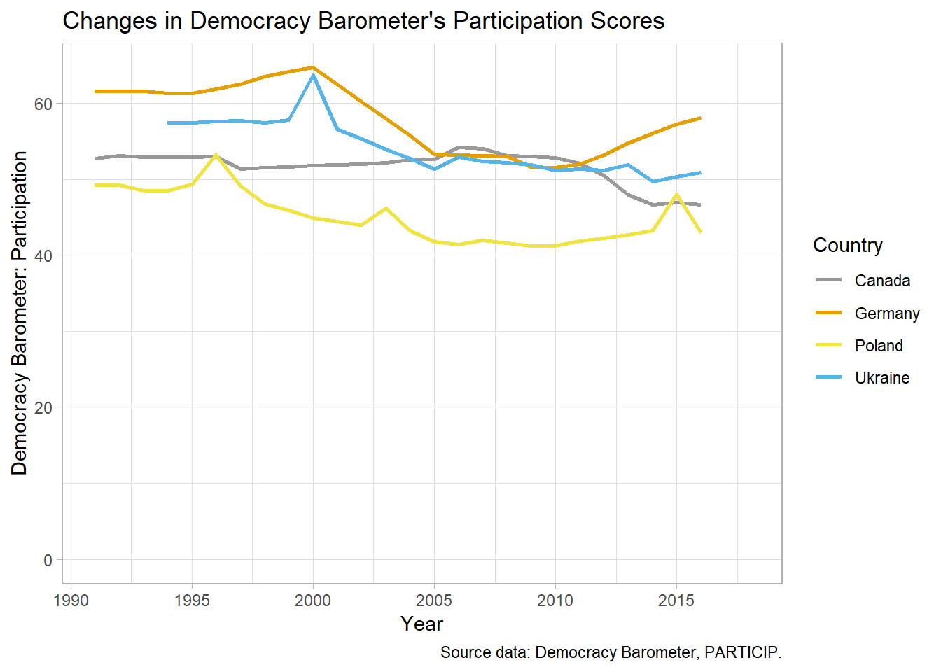

Variable graphs

The second graph shows changes in the same participation score and disposable income inequality (from teh SWIID) in Poland after 1990.

merged %>%
  filter(country %in% c("Poland"),
         year > 1990) %>%
  select(iso3, year, db_PARTICIP, gini_disp) %>%
  gather(variable, value, 3:4) %>%
  ggplot(., aes(x = year, y = value, col = variable)) +
  geom_line(size = 1) +
  ylab("Value") + expand_limits(y = 0) +
  scale_x_continuous(name = "Year",
                     breaks = seq(1990, 2015, 5)) +
  ggtitle("Changes in Democracy Barometer's Participation Scores and \nDisposable Income Inequality") +
  labs(caption = "Source data: Democracy Barometer, PARTICIP; SWIID, gini_disp.") +
  scale_color_manual(values = myPalette[1:2], 
                     name="Variable",
                     breaks = c("db_PARTICIP", "gini_disp"),
                     labels=c("Democracy Barometer \nParticipation", "Gini Disposable \nIncome")) +
  theme_light()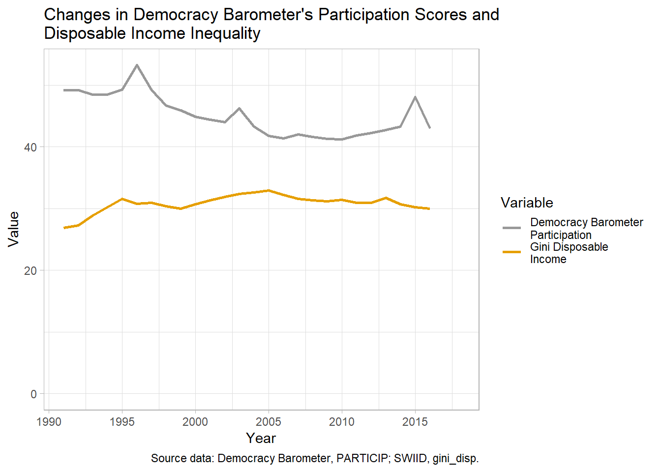

Writing to file

The final dataset can be saved to a CSV file for future use.

fwrite(merged, "merged.csv")