Introduction
Ex-post (or retrospective) data harmonization refers to procedures applied to already collected data to improve the comparability and inferential equivalence of measures collected by different studies. In practice, ex-post harmonization means a lot of recoding.
Reproducible recoding can be in form of code in some programming language, where running the code performs all the data transformations. When the number of recodes is large, the code quickly becomes long and complicated and difficult to follow for anyone but the code’s creator. I describe an alternative approach, developed during my work with Przemek Powałko on ex-post harmonization of income and voting variables, and a set of simple tools for the exploration, recoding, and documentation of harmonization of survey data, relying on crosswalks for mapping one coding scheme onto another. Recoding is then performed on the basis of the crosswalk mapping. This approach is used and further developed in the Survey Data Recycling project, which is moving from recoding with syntax to recoding based on crosswalks.
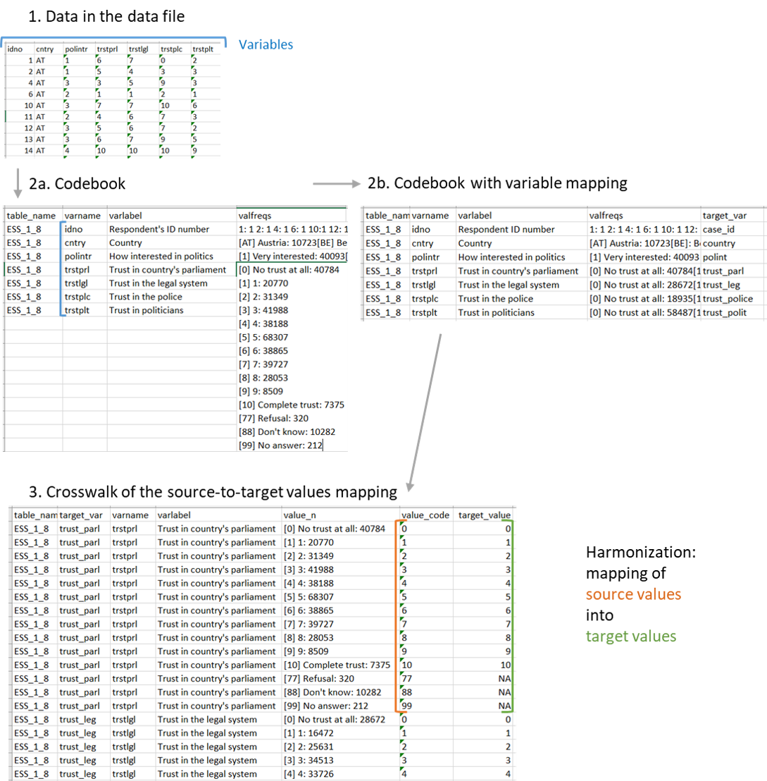
Figure 1 presents the data processing schema of the whole harmonization process. At the start (Step 1) there is a survey data file with cases (corresponding to respondents) in rows, and variables (corresponding to respondent characteristics) in columns. The survey data files’ metadata describing variables are used to construct the codebook (Step 2a), in which each row corresponds to a variable, and columns contain the original name of the variable in the survey data file as well as variable labels and value frequencies. Selected source variables corresponding to the concepts of interest are tagged with target variable names in a new column (Step 2b). Next, for the selected source variables a crosswalk is created, where for each value of each source variable there is a separate row. Assigning target variable values (Step 3) creates a mapping schema. This mapping schema is used in recoding of source to target variables, where a vector of source values is mapped onto a vector of target variables.
The full code is available here.

Figure 1: Harmonization: Data flow schema.
Illustration: Trust in institutions
As an illustration I use items on trust in institutions in three main cross-national survey projects in Europe: the European Social Survey (eight rounds in a single data file), the European Values Study (five rounds in two files), and the European Quality of Life Survey (four rounds in one file). The data are available from the project website, the GESIS archive, and the UK Data Archive, respectively.
All three projects conduct surveys in many European countries in each project wave, with samples intended as representative for entire adult populations of the respective country (in the ESS the minimum age is 15). Table 1 presents basic information about these survey projects. Standardized documentation about the methodology employed in all projects has been put together by Jabkowski’s Surveys Quality Assessment Database (SQAD) project.
| Project name | waves | data files | surveys | Years |
|---|---|---|---|---|
| European Social Survey (ESS) | 8 | 1 | 195 | 2002-2017 |
| European Quality of Life Survey (EQLS) | 4 | 1 | 126 | 2003-2016 |
| European Values Study (EVS) | 5 | 2 | 140 | 1981-2017 |
Trust in political and other institutions is a common item in many cross-national surveys and appears in all waves of all three projects. Each project includes questions about trust in a different set of institutions. Further, while in all three projects questionnaires tend to be relatively stable from wave to wave, the sets of questions have seen some changes, in particular new items had been added, and not always a given item was asked in all countries in a given wave. My goal is to see which trust items are the most, and which are the least popular in the three survey projects.
Step 1: Preparation and coding of technical variables
In the first step, all data files are loaded into the R workspace. The SPSS file format is preferred, since it comes with variable and value labels that are easy to extract. Next, the technical variables are identified, corresponding to the survey wave (if applicable), country, year, case (respondent) IDs, and weighting factors. A separate variable corresponds to the name of the source table. The code for data importing and preparation is shown in Appendix 1.
Step 2: Selection of source variables for harmonization
The second step in the harmonization process is the selection of source variables corresponding to the target concepts of interest. The target concepts in this case include trust in different institutions (as many as there are available in the source data), basic sociodemographics (age, gender, education, income), and selected covariates (satisfaction with life and social trust).
To map source variables to target variable names, the codebook is created with a list of source variables in each data set. This list should include the source variable name, and – since variable names tend to by cryptic – also the source variable label. The frequency distribution of values, as well as value labels, provide additional information in case the variable label is not informative, e.g., to distinguish age in years from age in categories.
In R, a codebook can be created from labelled data, such as those in SPSS format, with the package labelled. The R code for creating the codebook is presented in Appendix 2. The codebook is then exported into a spreadsheet program (e.g., with the rio package), where source variable labels can be browsed and filtered to select the variables of interest, and assign appropriate target variable names. The target variable names will be trust_*, where * is the short version of the institution name. If necessary, notes or comments on particular decisions can be written in a separate column of the spreadsheet. Notes may document decisions to treat questions about slightly different wording as corresponding to the same target variable (e.g., trust in the justice system vs. trust in the legal system), or add information from other sources, such as the original documentation of the source data.
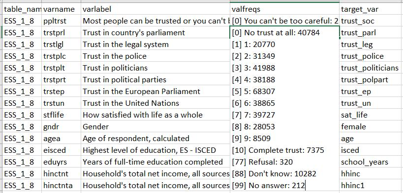
Figure 2 shows a snippet of the codebook created for ESS. The first column (table_name) corresponds to the name of the source table – one each for ESS and EQLS, and two separate tables for EVS/5 and EVS/1-4. The column varname contains the names of source variables, varlabel contains the source variable labels, and valfreqs contains frequencies of all values with value labels provided. The column target_var is to be filled with names of target variables to which the selected source variables correspond. In the example shown in Figure 2, the label trust_parl has been assigned to the variable on trust in parliament, the label trust_leg to the variable on trust in the legal system, and so on. Filtering available in spreadsheet programs enables sorting through variables with keywords or other conditions.

Figure 2: Codebook represented in a spreadsheet program.
Step 3: Mapping source values to target values
In the third step, for the variables selected in the codebook, a crosswalk template is created, where each value of each variable is in a separate row. Again, the labelled package can be used to obtain the desired format (code in Appendix 3).
This manual mapping of source values to target values, while mundane, achieves two goals. First, it enables the identification of missing value codes in each variable separately. Missing value codes are not always consistent even across variables in the same data set, and mistakes in automated recoding of missing values have a potentially large impact on the resulting data. Additionally, researchers might want to treat different missing values differently depending on their research goals, i.e., considering the “don’t know” category as a type of opinion (or rather lack thereof), and the “refusal” category as in fact missing.
The second goal is a careful inspection of labels of the source values, one by one, while consulting the textual survey documentation wherever necessary. The need to assign each target value a corresponding source value protects from possible mistakes of automation, and is particularly useful in the case of categorical variables with limited standardization across waves and projects, such as education or size of town of residence.
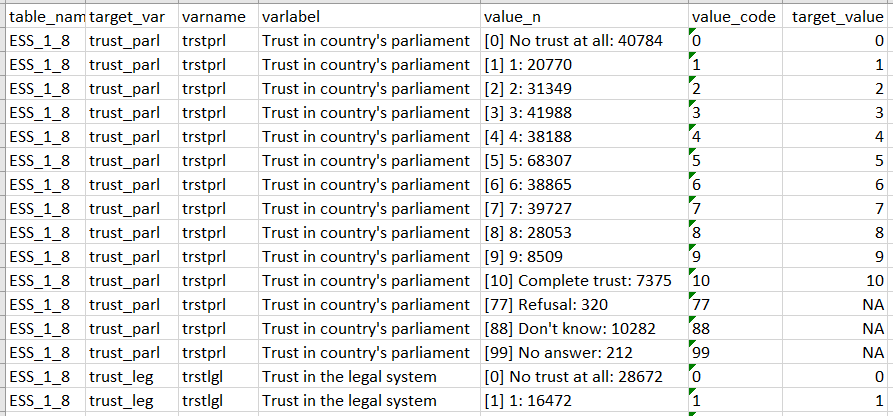
The snippet in Figure 3 shows a fragment of the crosswalk for trust in parliament in ESS, for which the source variable is called trstprl. Values include 77, 88, and 99 for different types of missing data, while values from 0 to 10 correspond to substantive answers. Corresponding target values are added in the target_value column.

Figure 3: Crosswalk represented in a spreadsheet program.
Step 4: Harmonization
Once the value crosswalk table is ready, it is imported into R, and – for each source variable separately – source and target values are extracted as vectors and used in data transformation. The function mapvalues from the plyr package, which maps each value from the source variable vector onto a corresponding value from the target variable vector, is particularly useful in this regard. The harmonization code is in Appendix 4.
Results: Availability of trust items
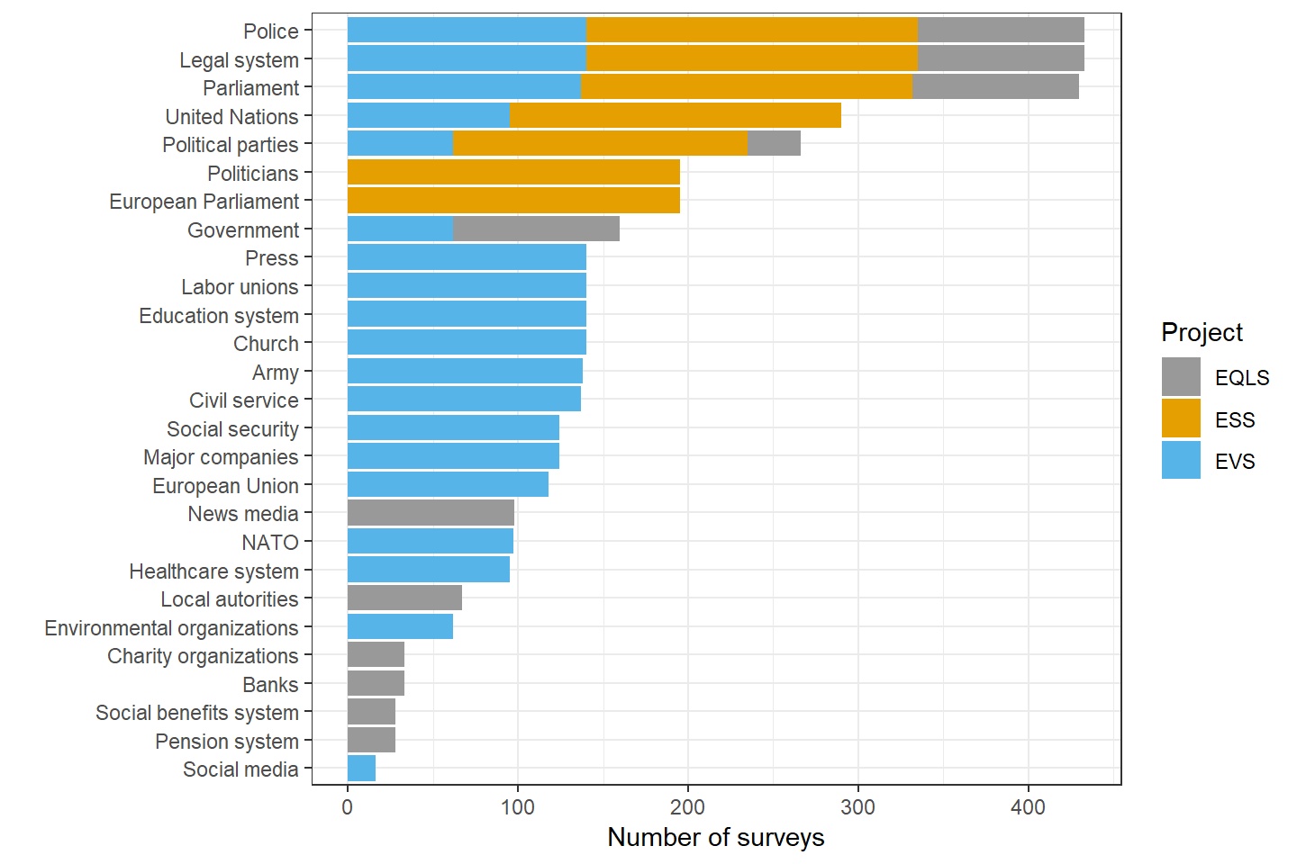
Altogether, in the three analyzed datasets, I identified trust items in 27 different institutions. The most common items are on trust in the legal system and in the police, available in 433 national surveys out of 461 surveys in total. The next item with regard to its availability in surveys is about trust in the national parliament (430 surveys), followed by trust in the United Nations (290) and trust in political parties (266). It is worth noting that I treated the European Union (118 surveys) and the European Parliament (195 surveys) as separate institutions. A different decision - combining both items into one target variable - would make it the fourth most popular turst item.
The availability of trust items across the three survey projects is presented in Figure 4. The three most common items – trust in the police, the legal system, and the national parliament – are available in all three projects: in all national surveys in ESS and EVS, and in rounds 2-4 of EQLS. The trust in parliament item is additionally missing from three surveys in EVS/2 (Estonia, Latvia, and Lithuania surveyed in 1990). Other items occur only in selected projects or project waves. For example, the item on trust in the social media was only added in EVS/5.

Figure 4: Availability of trust in institutions items in the European Social Survey Rounds 1-8, European Values Study 1-5, and the European Quality of Life Survey 1-4.
Comparability of sample aggregates
Caution is advised when comparing sample aggregates such as means or proportions obtained from different survey projects. A comparison of surveys carried out in the same country-years but in different projects shows substantial differences between samples, and these differences are difficult to explain away. An example of differences between levels of participation in demonstrations in the same countries and years but in different survey projects is described here.
Appendices: Code examples
Appendix 1: Data preparation
# EVS/5 (ZA7500_v1-0-0.sav.zip): https://dbk.gesis.org/dbksearch/GDESC2.asp?no=0009&DB=E
# EVS/1-4 (ZA4804_v3-0-0.sav.zip): https://dbk.gesis.org/dbksearch/GDESC2.asp?no=0009&DB=E
# ESS/1-8 (ESS1-8e01.zip): https://www.europeansocialsurvey.org/downloadwizard/
# EQLS/1-4 (eqls_integrated_trend_2003-2016.sav): https://beta.ukdataservice.ac.uk/datacatalogue/studies/study?id=7348

basic_vars <- c("table_name", "Tcountry", "Sid", "Tid", "Tweight", "Tround", "Tyear")

evs_2017 <- haven::read_sav("ZA7500_v1-0-0.sav.zip", user_na = TRUE) %>%
  mutate(Tcountry = c_abrv,
         Tid = row_number(),
         Sid = as.character(id_cocas),
         Tweight = 1,
         Tround = 5,
         table_name = "EVS_2017",
         Tyear = year,
         Tproject = "EVS")

evs_1981_2008 <- haven::read_sav("ZA4804_v3-0-0.sav.zip", user_na = TRUE) %>%
  mutate(Tcountry = S009,
         Tid = row_number(),
         Sid = as.character(S006),
         Tweight = S017,
         Tround = S002EVS,
         table_name = "EVS_1981_2008",
         Tyear = S020,
         Tproject = "EVS")

ess_1_8 <- haven::read_sav("ESS1-8e01.zip", user_na = TRUE) %>%
  mutate(Tcountry = cntry,
         Tid = row_number(),
         Sid = as.character(idno),
         Tweight = dweight * pspwght,
         table_name = "ESS_1_8",
         Tproject= "ESS",
         Tround = essround,
         Tyear = ifelse(is.na(inwyr), inwyys, inwyr),
         Tyear = ifelse(Tyear == 9999, NA, Tyear)) %>%
  group_by(essround, cntry) %>%
  mutate(Tyear = round(mean(Tyear, na.rm = TRUE)),
         Tyear = ifelse(cntry == "EE" & essround == 5, 2011, Tyear)) %>%
  ungroup()

eqls_1_4 <- haven::read_sav("eqls_integrated_trend_2003-2016.zip", user_na = TRUE) %>%
  mutate(Tcountry = plyr::mapvalues(Y16_Country,
                                     c(1:36),
                                     c("AT", "BE", "BG", "CY", "CZ", "DE", "DK", "EE", "GR", "ES",
                                       "FI", "FR", "HR", "HU", "IE", "IT", "LT", "LU", "LV", "MT",
                                       "NL", "PL", "PT", "RO", "SE", "SI", "SK", "UK", "AL", "IS",
                                       "KS", "ME", "MK", "NO", "RS", "TR")),
         Tid = row_number(),
         Sid = as.character(Y16_uniqueid),
         Tweight = WCalib,
         Tround = Wave,
         Tyear = plyr::mapvalues(Wave, c(1,2,3,4), c(2003, 2007, 2011, 2016)),
         table_name = "EQLS_1_4",
         Tproject = "EQLS")

### dealing with non-unique labels in evs_1981_2008
# Thanks to: https://dadoseteorias.wordpress.com/2017/04/29/read-spss-duplicated-levels/
Int2Factor <- function(x)
{
  if(!is.null(attr(x, "value.labels"))){
    vlab <- attr(x, "value.labels")
    if(sum(duplicated(vlab)) > 0)
      cat("Duplicated levels:", vlab, "\n")
    else if(sum(duplicated(names(vlab))) > 0)
      cat("Duplicated labels:",
          names(vlab)[duplicated(names(vlab))], "\n")
    else
      x <- factor(x, levels = as.numeric(vlab),
                  labels = names(vlab))
  }
  x
}

evs_1981_2008 <- lapply(evs_1981_2008, Int2Factor) %>% as.data.frame(., stringsAsFactors = FALSE)
Appendix 2: Codebook from labelled data in R
create_codebook <- function(data) {
  var_labels <- data.frame(cbind(names(var_label(data)), do.call(rbind, var_label(data)))) %>%
    rename(varname = X1, varlabel = X2)

  freqs <- lapply(data, function(x) { return(questionr::freq(x)) }) %>%
    keep(function(x) nrow(x) < 1000) %>%
    do.call(rbind, .) %>%
    tibble::rownames_to_column(var = "varname_value") %>%
    mutate(varname = gsub("(.+?)(\\..*)", "\\1", varname_value),
           value = gsub("^[^.]*.","",varname_value)) %>%
    group_by(varname) %>%
    mutate(npos = row_number(),
           value_n = paste(value, n, sep = ": ")) %>%
    select(varname, value_n, npos) %>%
    spread(npos, value_n) %>%
    mutate_at(vars(-varname), funs(ifelse(is.na(.), "", .))) %>%
    unite("valfreqs", c(2:ncol(.)), sep = "\n") %>%
    mutate(valfreqs = sub("\\s+$", "", valfreqs))

  full_join(var_labels, freqs, by = "varname")
}

codebook_evs_2017 <- create_codebook(evs_2017) %>%
  mutate(table_name = "EVS_2017")
codebook_evs_1981_2008 <- create_codebook(evs_1981_2008) %>%
 mutate(table_name = "EVS_1981_2008")
codebook_eqls_1_4 <- create_codebook(eqls_1_4) %>%
  mutate(table_name = "EQLS_1_4")
codebook_ess_1_8 <- create_codebook(ess_1_8) %>%
  mutate(table_name = "ESS_1_8")

codebook_all <- bind_rows(codebook_ess_1_8, codebook_evs_1981_2008,
                          codebook_evs_2017, codebook_eqls_1_4) %>%
  mutate(target_var = NA)

rio::export(codebook_all, "codebook_all.xlsx")
Appendix 3: Values crosswalk
codebook_all1 <- rio::import("codebook_all1.xlsx") %>%
  filter(!is.na(target_var))

create_cwt <- function(data) {

  var_labels <- data.frame(cbind(names(var_label(data)), do.call(rbind, var_label(data)))) %>%
    rename(varname = X1, varlabel = X2)

  freqs_cwt <- lapply(data, function(x) { return(questionr::freq(x)) }) %>%
    keep(function(x) nrow(x) < 1000) %>%
    do.call(rbind, .) %>%
    tibble::rownames_to_column(var = "varname_value") %>%
    mutate(varname = gsub("(.+?)(\\..*)", "\\1", varname_value),
           value = gsub("^[^.]*.","",varname_value),
           value_code = sub(".*\\[(.+)\\].*", "\\1", varname_value, perl = TRUE),
           value_code = ifelse(str_sub(varname_value, -2, -1) == "NA", "NA", value_code),
           value_code = ifelse(gsub(" ", "", fixed = TRUE, varname_value) == varname_value,
                               gsub("^[^.]*.","",varname_value), value_code)) %>%
    group_by(varname) %>%
    mutate(npos = row_number(),
           value_n = paste(value, n, sep = ": ")) %>%
    select(npos, varname, value_n, value, value_code)

  full_join(var_labels, freqs_cwt, by = "varname")
}

data_tables <- c("EVS_2017", "EVS_1981_2008", "EQLS_1_4", "ESS_1_8")
cwt_all <- list()

for (i in (1:length(data_tables))) {

  table_name_input <- data_tables[i]
  varnames <- codebook_all1$varname[codebook_all1$table_name == table_name_input]

  cwt_all[[i]] <- eval(parse(text = tolower(table_name_input))) %>%
    select(varnames) %>%
    create_cwt() %>%
    mutate(table_name = table_name_input)
}

cwt_all <- do.call(rbind, cwt_all)

cwt_all %>%
  select(-varlabel) %>%
  left_join(codebook_all1, by = c("varname", "table_name")) %>%
  mutate(target_value = NA) %>%
  select(table_name, target_var,
         varname, varlabel, starts_with("c_"),
         value_n, value_code, target_value) %>%
  rio::export(., "cwt_all.xlsx")
Appendix 4: Harmonization
cwt_all1 <- rio::import("cwt_all1.xlsx")

harmonize <- function(table_name_input, cwt_name_input) {

  target_vars <- unique(eval(parse(text = tolower(cwt_name_input)))$target_var[eval(parse(text = tolower(cwt_name_input)))$table_name == table_name_input])
  source_vars <- unique(eval(parse(text = tolower(cwt_name_input)))$varname[eval(parse(text = tolower(cwt_name_input)))$table_name == table_name_input])

  data_small <- eval(parse(text = tolower(table_name_input))) %>%
    select(basic_vars, source_vars) %>%
    zap_labels()

  harmonized_vars <- list()

  for (i in 1:length(target_vars)) {

    target_var_input = target_vars[i]

    source <- eval(parse(text = tolower(cwt_name_input))) %>%
      filter(target_var == target_var_input, table_name == table_name_input) %>%
      pull(value_code)

    target <- eval(parse(text = tolower(cwt_name_input))) %>%
      filter(target_var == target_var_input, table_name == table_name_input) %>%
      pull(target_value)

    source_varname <- eval(parse(text = tolower(cwt_name_input))) %>%
      filter(target_var == target_var_input, table_name == table_name_input) %>%
      pull(varname) %>% .[1]

    harmonized_vars[[i]] <- data_small %>%
      mutate(!!target_var_input := as.numeric(plyr::mapvalues(as.character(get(source_varname)),
                                                              source, target))) %>%
      select(basic_vars, target_var_input)
  }
  Reduce(merge,harmonized_vars)
}

evs_2017_h <- harmonize("EVS_2017", "cwt_all1")
  rm(evs_2017) # remove original data files from work space
evs_1981_2008_h <- harmonize("EVS_1981_2008", "cwt_all1")
  rm(evs_1981_2008)
ess_1_8_h <- harmonize("ESS_1_8", "cwt_all1")
  rm(ess_1_8)
eqls_1_4_h <- harmonize("EQLS_1_4", "cwt_all1")
  rm(eqls_1_4)

all_data <- bind_rows(evs_2017_h, evs_1981_2008_h,
                      ess_1_8_h, eqls_1_4_h) %>%
  mutate(Tproject = sub("\\_.*", "", table_name)) %>%
  select(table_name, starts_with("T", ignore.case = FALSE),
         starts_with("S", ignore.case = FALSE), everything())

rio::export(all_data, "harmonization-europe-trust.csv.gz") 