
The 2020 paper “Deprivation in the Midst of Plenty: Citizen Polarization and Political Protest” by Griffin, Kiewiet de Jonge, and Velasco-Guachalla, published by in British Journal of Political Science, contains a data error that invalidates the study’s main results and conclusions that polarization leads to higher protest activity. The error is quite trivial and lies in the construction of the dependent variable of the study. After fixing the data error the results no longer indicate a positive effect of polarization on protest, nor a moderating effect of grievances.
The paper’s original replication materials are in this Dataverse repository.
I starts with a brief summary of the theoretical argument and the data and measures used. Next, I explain the source of the error, reproduce the original analysis and present the corrected analyses after the data error is fixed.
Summary of Griffin et al.
The theoretical argument builds on Ted Gurr’s grievance theory to argue that the main determinant of protest is not the level of grievances itself, but the polarization of grievances. High polarization of grievances, i.e. a situation when some groups in a society are very dissatisfied, while others are very satisfied, is conducive to protest eruption because it implies feelings of relative deprivation among the dissatisfied group, who compare themselves to the satisfied groups.
The scope conditions, according to the authors, include the requirement of a democratic context, and - relatedly - peaceful anti-government protest rather than collective violence.
The measure of polarization is constructed as a sample standard deviation of responses to the question about satisfaction with democracy from various cross-national survey projects. It is measured at the country-year level.
The level of protest is measured as the number of anti-government protests and strikes at the country-year level, taken from the Cross National Time Series (CNTS) dataset. It too is measured at the country-year level.
Data inspection
I should note that I have not attempted to reproduce the measure of polarization, nor have I paid much attention to how the control variables were constructed. I just focus on the protest measure, i.e. the dependent variable of the study.
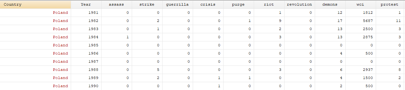
The file Conflict data sample in the replication materials
contains the protest data used in the article to construct the dependent variable.
Here is a snippet for Poland 1981-1990.
The variable protest is the one created by the authors and used in the analysis.
In the article, it is described as the
sum of strikes (strike) and anti-government demonstrations (demons).
It is enough to eyeball the data to see that the variable ‘protest’ is not a sum of
strike and demons. Rather, the variable protest looks like strike + riot.
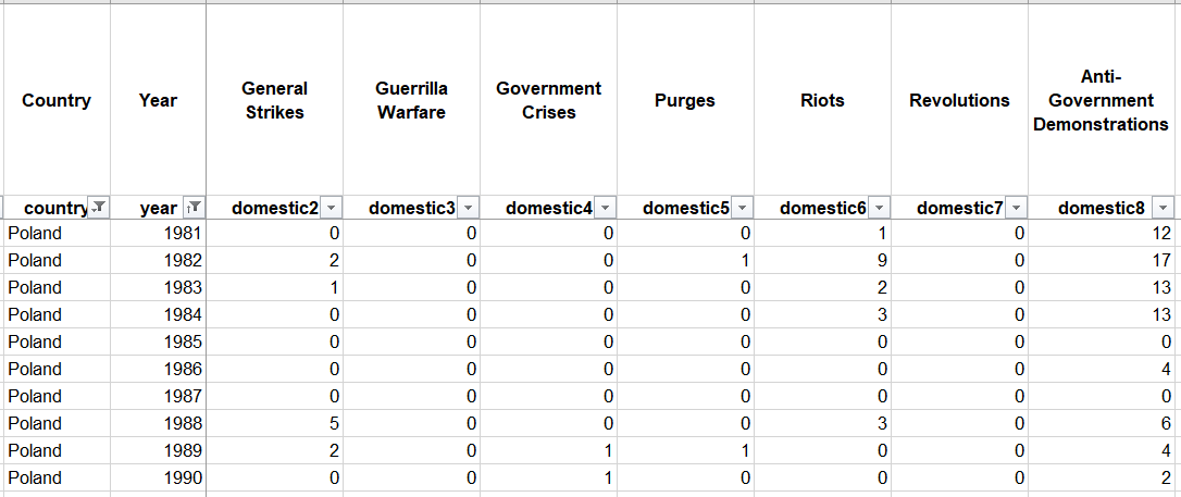
I checked the original CTNS data downloaded following instructions on the CTNS project website. Below is the data snippet for Poland in 1981-1990. The counts of demonstrations, riots, and strikes registered in Poland 1981-1990 match the numbers in the Griffin et al. replication data file.
The error in creating the protest variable looks trivial.
The authors must have added together the wrong data columns. This is an easy mistake to make
if the CTNS data are imported into data analysis software with only the short variable
names (domestic2, domestic3, …) and not full labels.
Reanalysis
I start by downloading the data files from the authors’ Dataverse repository.
library(tidyverse) # for manipulating data
library(dataverse) # for getting data from Dataverse
library(zoo) # for interpolating
library(skimr) # for making quick data summarise
library(kableExtra) # for making tables
library(glmmTMB) # for running generalized linear mixed models
library(sjPlot) # model tables (and much more!)

# Polarization dataset
polarization <- get_dataframe_by_name(
  filename = "Polarization dataset.tab",
  dataset = "10.7910/DVN/SVXE7L",
  server = "dataverse.harvard.edu")

# Protest dataset
conflict <- get_dataframe_by_name(
  filename = "Conflict data sample.tab",
  dataset = "10.7910/DVN/SVXE7L",
  server = "dataverse.harvard.edu")

# Control variables dataset
qog <- get_dataframe_by_name(
  filename = "QOG sample.tab",
  dataset = "10.7910/DVN/SVXE7L",
  server = "dataverse.harvard.edu")
The code below is a translation of the Stata code in Polarization_Protest models.do
from the replication materials to R.
combo <- polarization %>%
  # merge all datasets by country and year
  full_join(conflict, by = c("ccode", "Year")) %>%
  full_join(qog, by = c("ccode", "Year")) %>%
  mutate(# correct measure of anti-gov demonstrations + strikes
         demons_strike = demons + strike,
         # riots + strikes
         riot_strike = riot + strike,
         # other transformations as in the original data cleaning script
         polar = polar*100,
         disat = disat*100,
         GDPcap = log(pwt_rgdpch),
         Growth = wdi_gdpgr,
         Inflation = wdi_infl,
         Ln_Inflation = ifelse(Inflation >= 1, log(Inflation), 0),
         polity2 = p_polity2,
         Eth_frag = al_ethnic,
         Ln_pop = log(wdi_pop),
         Elec_leg = dpi_legelec,
         Elec_exe = dpi_exelec,
         ENP = gol_enpp,
         Presidential = as.numeric(dpi_system == 0),
         Presidential = ifelse(is.na(dpi_system), 0, Presidential),
         Urban = wdi_urban,
         reg_durability = p_durable,
         terror = gd_ptss,
         timetrend = Year - 2000
         ) %>%
  arrange(Country, Year) %>%
  group_by(Country) %>%
  # interpolate income inequality
  mutate(gini = zoo::na.approx(solt_ginet, na.rm = F)) %>%
  ungroup() %>%
  # keep democracies only
  filter(polity2 >= 0) %>%
  # created lagged and centered variables
  mutate_at(vars(protest, demons_strike, riot_strike, demons, riot, strike, polar, disat, gini,
                 GDPcap, Growth, Inflation, Ln_Inflation, Elec_leg, Elec_exe, polity2, reg_durability,
                 terror, Urban, Ln_pop),
            .funs = list(l = ~lag((. - mean(., na.rm = T)), 1))) %>%
  # drop cases with missing lagged polarization
  drop_na(polar_l) %>%
  select(ccode, Year, demons_strike, demons_strike_l, riot_strike, riot_strike_l,
         protest, protest_l, polar_l, disat_l, gini_l, GDPcap_l,
         Growth_l, Ln_Inflation_l, Elec_leg_l, Elec_exe_l, polity2_l,
         reg_durability_l, terror_l, Urban_l, Ln_pop_l, Presidential,
         Eth_frag, timetrend)
Here’s the summary of all relevant variables. Note that the protest variable,
constructed by the Griffin et al., and the riot_strike variable, constructed by myself
as a sum of the number of riots and strikes, are the same.
skimr::skim(combo) %>%
  mutate(numeric.mean = round(numeric.mean, 3)) %>%
  mutate(numeric.sd = round(numeric.sd, 3)) %>%
  mutate(numeric.p0 = round(numeric.p0, 3)) %>%
  mutate(numeric.p100 = round(numeric.p100, 3)) %>%
  dplyr::select(skim_variable, n_missing, numeric.mean, numeric.sd, numeric.p0, numeric.p100) %>%
  print(n = 25)
## # A tibble: 24 × 6
## skim_variable n_missing numeric.mean numeric.sd numeric.p0 numeric.p100
## <chr> <int> <dbl> <dbl> <dbl> <dbl>
## 1 ccode 0 412. 245. 8 894
## 2 Year 0 2000. 9.36 1967 2011
## 3 demons_strike 71 0.784 1.63 0 12
## 4 demons_strike_l 27 -0.145 1.58 -0.928 11.1
## 5 riot_strike 72 0.439 1.33 0 22
## 6 riot_strike_l 28 -0.256 1.21 -0.672 21.3
## 7 protest 71 0.439 1.33 0 22
## 8 protest_l 27 -0.256 1.21 -0.672 21.3
## 9 polar_l 0 0 6.26 -17.5 31.0
## 10 disat_l 0 0 8.53 -24.0 22.5
## 11 gini_l 107 -2.68 9.80 -18.9 28.8
## 12 GDPcap_l 34 0.439 0.93 -3.21 1.94
## 13 Growth_l 12 -0.651 4.79 -48.3 14.9
## 14 Ln_Inflation_l 12 -0.209 1.32 -1.94 6.77
## 15 Elec_leg_l 9 0.024 0.454 -0.266 0.734
## 16 Elec_exe_l 8 0.009 0.334 -0.118 0.882
## 17 polity2_l 0 0.877 1.79 -7.82 2.18
## 18 reg_durability_l 0 0.913 31.8 -29.7 171.
## 19 terror_l 22 -0.241 0.984 -1.14 2.86
## 20 Urban_l 5 8.61 15.0 -45.5 38.5
## 21 Ln_pop_l 5 0.105 1.26 -3.23 4.54
## 22 Presidential 0 0.394 0.489 0 1
## 23 Eth_frag 0 0.313 0.216 0.002 0.93
## 24 timetrend 0 -0.211 9.36 -33 11And here is a summary of the data created with the authors’ original code. The summary statistics in the table below are the same as in the table above, up to rounding error.
 Variable           Obs        Mean    Std. Dev.       Min        Max
 protest            971     .438723    1.333588          0         22
 l_protest        1,015   -.2562795    1.213236   -.672043   21.32796
 l_polar          1,042    3.51e-07    6.258634  -17.48873   31.01496
 l_disat          1,042    3.33e-06    8.526368  -23.96803   22.46431
 l_gini             935   -2.684602    9.803594  -18.88194   28.81756
 l_GDPcap         1,008    .4393539     .930272  -3.211872   1.935358
 l_Growth         1,030   -.6509732    4.790745  -48.32703   14.85958
 l_Ln_Inflation   1,030   -.2092084    1.322055  -1.936994    6.76943
 l_Elec_leg       1,033    .0243469    .4541744  -.2660694   .7339306
 l_Elec_exe       1,034    .0092795    .3338718  -.1183801   .8816199
 l_polity2        1,042    .8766785    1.792215   -7.81622    2.18378
 l_reg_durability 1,042    .9132185    31.78594  -29.67699    171.323
 l_terror         1,020   -.2409006    .9839658  -1.144822   2.855178
 l_Urban          1,037    8.612539    15.04106  -45.52881   38.51258
 l_Ln_pop         1,037    .1051592    1.261732  -3.233301   4.535833
 Presidential     1,042    .3944338    .4889634          0          1
 Eth_frag         1,042    .3128498    .2159714    .001998    .930175
 timetrend        1,042   -.2111324    9.355481        -33         11
Results
The authors estimate negative binomial count models predicting the number of events. They present both “flat” models with errors clustered by country and multilevel models with country-years nested in countries. I focus on the latter.
Main effects
The code below reproduces Model specification 2 with country random effects from
Table 1 in Griffin et al. - model protest in the output table below. The second model
replaces the original protest variable with the sum of counts of demonstrations and
strikes, demons_strike.
The crucial coefficient is the effect of lagged polarization,
polar_l. In the original model the coefficient is estimated at 0.046, significant at
the 0.05 level. In the corrected model the coefficient equals 0.009 and is no longer significant.
Note that not all coefficient values of the protest model below are exactly the same as
in the original table in Griffin et al. For example, the coefficient for lagged protest
in the reanalysis below is 0.197, SE = 0.065,
compared to 0.195, SE = 0.065 in the Griffin et al. paper. This is likely due to small differences in
the estimation routine menbreg in Stata and in the R package glmmTMB.
Coefficients for the effects of polarization are the same whether the model is estimated
in R or Stata, and equal 0.009 with SE = 0.015.
re_original <- glmmTMB(protest ~ protest_l + polar_l + disat_l +
                         gini_l + I(gini_l^2) + GDPcap_l + Growth_l + Ln_Inflation_l +
                         Elec_leg_l + Elec_exe_l + polity2_l + reg_durability_l +
                         terror_l + Urban_l + Ln_pop_l + Presidential + Eth_frag + timetrend +
                  (1 | ccode),
                  data = combo,
                  ziformula = ~0,
                  family = nbinom2)

re_corrected <- glmmTMB(demons_strike ~ demons_strike_l + polar_l + disat_l +
                          gini_l + I(gini_l^2) + GDPcap_l + Growth_l + Ln_Inflation_l +
                          Elec_leg_l + Elec_exe_l + polity2_l + reg_durability_l +
                          terror_l + Urban_l + Ln_pop_l + Presidential + Eth_frag + timetrend +
                  (1 | ccode),
                  data = combo,
                  ziformula = ~0,
                  family = nbinom2)

sjPlot::tab_model(re_original, re_corrected, show.ci = FALSE, show.se = TRUE, transform = NULL,
                  digits = 3, emph.p = FALSE,
order.terms = c(2,20,3:19,1))| protest | demons strike | |||||
|---|---|---|---|---|---|---|
| Predictors | Log-Mean | std. Error | p | Log-Mean | std. Error | p |
| protest l | 0.197 | 0.065 | 0.003 | |||
| demons strike l | 0.125 | 0.042 | 0.003 | |||
| polar l | 0.046 | 0.019 | 0.015 | 0.009 | 0.015 | 0.548 |
| disat l | -0.000 | 0.015 | 0.977 | 0.016 | 0.011 | 0.151 |
| gini l | 0.020 | 0.021 | 0.340 | 0.034 | 0.016 | 0.037 |
| gini l^2 | -0.000 | 0.001 | 0.831 | 0.000 | 0.001 | 0.812 |
| GDPcap l | -0.222 | 0.315 | 0.481 | -0.135 | 0.239 | 0.570 |
| Growth l | -0.024 | 0.023 | 0.280 | -0.001 | 0.018 | 0.974 |
| Ln Inflation l | -0.087 | 0.102 | 0.392 | -0.102 | 0.079 | 0.194 |
| Elec leg l | 0.199 | 0.201 | 0.324 | 0.182 | 0.158 | 0.250 |
| Elec exe l | 0.080 | 0.292 | 0.783 | 0.329 | 0.218 | 0.131 |
| polity2 l | -0.119 | 0.073 | 0.105 | -0.161 | 0.057 | 0.005 |
| reg durability l | -0.004 | 0.006 | 0.485 | -0.004 | 0.005 | 0.363 |
| terror l | -0.052 | 0.147 | 0.725 | -0.076 | 0.117 | 0.514 |
| Urban l | 0.027 | 0.014 | 0.048 | 0.019 | 0.010 | 0.060 |
| Ln pop l | 0.395 | 0.116 | 0.001 | 0.411 | 0.090 | <0.001 |
| Presidential | -0.593 | 0.461 | 0.199 | -0.408 | 0.354 | 0.249 |
| Eth frag | -0.284 | 0.782 | 0.716 | -0.432 | 0.600 | 0.472 |
| timetrend | -0.038 | 0.015 | 0.011 | -0.030 | 0.012 | 0.012 |
| (Intercept) | -1.341 | 0.425 | 0.002 | -0.614 | 0.337 | 0.069 |
| Random Effects | ||||||
| σ2 | 2.07 | 1.57 | ||||
| τ00 | 0.53 ccode | 0.31 ccode | ||||
| ICC | 0.20 | 0.16 | ||||
| N | 84 ccode | 84 ccode | ||||
| Observations | 874 | 874 | ||||
| Marginal R2 / Conditional R2 | 0.244 / 0.397 | 0.303 / 0.417 | ||||
Moderation
I now turn to model specification 3 with country random effects, which adds an interaction between polarization and dissatisfaction. The first model reproduces the one from the paper, the second one corrects the data error.
In the reproduction the main effect of polarization is 0.044, SE = 0.019, significant at the 0.05 level. The interaction effect equals -0.004, SE = 0.002, significant at the 0.1 level, like in the published paper.
After correcting the data error the main effect of polarization and the interaction effect become much smaller and neither is statistically significant.
re_original_mod <- glmmTMB(protest ~ protest_l + polar_l*disat_l +
                         gini_l + I(gini_l^2) + GDPcap_l + Growth_l + Ln_Inflation_l +
                         Elec_leg_l + Elec_exe_l + polity2_l + reg_durability_l +
                         terror_l + Urban_l + Ln_pop_l + Presidential + Eth_frag + timetrend +
                  (1 | ccode),
                  data = combo,
                  ziformula = ~0,
                  family = nbinom2)

re_corrected_mod <- glmmTMB(demons_strike ~ demons_strike_l + polar_l*disat_l +
                          gini_l + I(gini_l^2) + GDPcap_l + Growth_l + Ln_Inflation_l +
                          Elec_leg_l + Elec_exe_l + polity2_l + reg_durability_l +
                          terror_l + Urban_l + Ln_pop_l + Presidential + Eth_frag + timetrend +
                  (1 | ccode),
                  data = combo,
                  ziformula = ~0,
                  family = nbinom2)

sjPlot::tab_model(re_original_mod, re_corrected_mod, show.ci = FALSE, show.se = TRUE, transform = NULL,
                  digits = 3, emph.p = FALSE,
order.terms = c(2,21,3,4,20,5:19,1))| protest | demons strike | |||||
|---|---|---|---|---|---|---|
| Predictors | Log-Mean | std. Error | p | Log-Mean | std. Error | p |
| protest l | 0.198 | 0.065 | 0.002 | |||
| demons strike l | 0.127 | 0.042 | 0.002 | |||
| polar l | 0.044 | 0.019 | 0.017 | 0.009 | 0.015 | 0.550 |
| disat l | 0.008 | 0.015 | 0.589 | 0.019 | 0.012 | 0.111 |
| polar l × disat l | -0.004 | 0.002 | 0.060 | -0.001 | 0.002 | 0.454 |
| gini l | 0.021 | 0.021 | 0.315 | 0.035 | 0.016 | 0.034 |
| gini l^2 | -0.000 | 0.001 | 0.962 | 0.000 | 0.001 | 0.786 |
| GDPcap l | -0.253 | 0.309 | 0.414 | -0.140 | 0.237 | 0.555 |
| Growth l | -0.031 | 0.023 | 0.172 | -0.002 | 0.018 | 0.898 |
| Ln Inflation l | -0.096 | 0.101 | 0.345 | -0.103 | 0.079 | 0.192 |
| Elec leg l | 0.218 | 0.201 | 0.278 | 0.188 | 0.158 | 0.234 |
| Elec exe l | 0.056 | 0.290 | 0.846 | 0.324 | 0.218 | 0.136 |
| polity2 l | -0.098 | 0.073 | 0.176 | -0.154 | 0.057 | 0.007 |
| reg durability l | -0.003 | 0.006 | 0.665 | -0.004 | 0.005 | 0.430 |
| terror l | -0.029 | 0.147 | 0.842 | -0.072 | 0.116 | 0.536 |
| Urban l | 0.027 | 0.013 | 0.043 | 0.019 | 0.010 | 0.059 |
| Ln pop l | 0.408 | 0.114 | <0.001 | 0.412 | 0.089 | <0.001 |
| Presidential | -0.627 | 0.451 | 0.165 | -0.417 | 0.351 | 0.235 |
| Eth frag | -0.409 | 0.772 | 0.596 | -0.469 | 0.597 | 0.432 |
| timetrend | -0.037 | 0.015 | 0.011 | -0.030 | 0.012 | 0.012 |
| (Intercept) | -1.286 | 0.416 | 0.002 | -0.591 | 0.335 | 0.077 |
| Random Effects | ||||||
| σ2 | 2.07 | 1.57 | ||||
| τ00 | 0.47 ccode | 0.29 ccode | ||||
| ICC | 0.19 | 0.16 | ||||
| N | 84 ccode | 84 ccode | ||||
| Observations | 874 | 874 | ||||
| Marginal R2 / Conditional R2 | 0.266 / 0.403 | 0.308 / 0.417 | ||||
Conclusion
After fixing the data error the above analysis fails to provide evidence that polarization (or dispersion) of satisfaction with democracy predicts the total number of anti-government demonstrations and strikes.
The error needs to be corrected. I contacted the authors in January 2024 and BJPS in May 2024, and nothing has been done yet.