Note: This part of data processing was used to construct poststratification tables used to create country-year estimates of political trust in Europe. The full paper titled “Modeling public opinion over time and space: Trust in state institutions in Europe, 1989-2019” is availabe on SocArXiv: https://osf.io/preprints/socarxiv/3v5g7/. This research was supported by the Bekker Programme of the Polish National Agency for Academic Mobility under award number PPN/BEK/2019/1/00133.
The Eurostat provides a host of useful data, including socio-demographic statistics on educational attainment, which enable tracking the changes in educational composition of European societies over the last several years.
Eurostat’s lfsa_pgaed time series titled “Population by sex, age and educational attainment level (1 000)” provides population counts by education level (ISCED 0-2, 3-4, 5-8), gender (male and female) and age group (several different groupings). The data are aggregated from the European Labor Force Surveys, EU-LFS. EU-LFS micro-data require special permissions, but the aggregated tables provided by the Eurostat can be used freely as far as one is happy with the groupings and other limitations.
Like all publicly available data from the Eurostat, the education time series can be downloaded using the eurostat package.
The excerpt below show the first few rows of the table: The unit is thousand people, sex is coded as F for female and M for male, age is coded as “Y” and then the age range, education as “ED” and ISCED 2011 levels, geo indicates the country, time indicates the year, and values provide the population counts (in thousands).
library(eurostat) # for getting data from the Eurostat
library(sjlabelled) # for dealing with variable and value labels
library(countrycode) # for switching between country code types
library(tidyverse) # for manipulating data
library(viridis) # for color palettes

edu_raw <- get_eurostat("lfsa_pgaed",
                        time_format = "num",
                        stringsAsFactors = FALSE)

head(edu_raw)
## # A tibble: 6 x 7
## unit sex age isced11 geo time values
## <chr> <chr> <chr> <chr> <chr> <dbl> <dbl>
## 1 THS F Y15-19 ED0-2 AT 2019 150.
## 2 THS F Y15-19 ED0-2 BE 2019 243.
## 3 THS F Y15-19 ED0-2 BG 2019 124.
## 4 THS F Y15-19 ED0-2 CH 2019 166.
## 5 THS F Y15-19 ED0-2 CY 2019 17.5
## 6 THS F Y15-19 ED0-2 CZ 2019 202.The data are provided starting from 1983 for 10 countries and reach 35 EU and candidate countries countries in 2010-2019.
The table would be ready to be used as is, but for unclear reasons data for some categories are missing, even though in other categories and total are available. For example, for Estonia in 2004, for the age group 20-24 and the education category ED0-2, information is provided about the number of men and the total number of people, but information for women is not provided. There are several other cases with regard to gender, as well as education and age groups that should be corrected in order to make the data more complete.
edu <- edu_raw %>%
  spread(isced11, values) %>%
  # filter out the youngest age group
  filter(age != "Y15-19",
         # keep year since 1990
         time >= 1990) %>%
  rename(`ED3-4` = `ED3_4`) %>%
  # calculate ED5-8 from total and ED0-2 and ED3-4 if missing
  mutate(`ED5-8` = ifelse(is.na(`ED5-8`),
                          TOTAL - NRP - `ED0-2` - `ED3-4`,
                          `ED5-8`)) %>%
  # reshape to long
  gather(isced11, values, 6:10) %>%
  # keep only the categories of interest
  filter(isced11 %in% c("ED0-2", "ED3-4", "ED5-8")) %>%
  # select columsn to keep
  select(geo, time, age, sex, isced11, nobs_cat = values) %>%
  spread(sex, nobs_cat) %>%
  # fill in M or F, if missing, by using the total and non-missing category
  mutate(M = ifelse(is.na(M), T - F, M),
         F = ifelse(is.na(F), T - M, F)) %>%
  gather(sex, nobs_cat, 5:7) %>%
  filter(sex != "T") %>%
  spread(age, nobs_cat) %>%
  # fill in age groups, if missing, with info from other categories
  mutate(`Y35-39` = ifelse(is.na(`Y35-39`), `Y25-39` - `Y25-29` - `Y30-34`, `Y35-39`),
         `Y40-44` = ifelse(is.na(`Y40-44`), `Y40-59` - `Y45-49` - `Y50-59`, `Y40-44`),
         `Y70-74` = `Y50-74`-(`Y50-54`+`Y55-64`+`Y65-69`),
         `Y20-34` = `Y20-24`+`Y25-29`+`Y30-34`,
         `Y35-54` = `Y35-39`+`Y40-44`+`Y45-49`+`Y50-54`,
         `Y55-74` = `Y55-64`+`Y65-69` + `Y70-74`) %>%
  select(geo, time, sex, isced11, `Y20-34`, `Y35-54`, `Y55-74`) %>%
  gather(age_cat, nobs_cat, 5:7) %>%
  group_by(geo, time, sex, age_cat) %>%
  mutate(prop_cat = nobs_cat / sum(nobs_cat)) %>%
  ungroup() %>%
  select(geo, time, age_cat, sex, isced11, prop_cat) %>%
  arrange(geo, time, age_cat, sex, isced11)

edu %>%
  filter(geo == "PL") %>%
  head(6)
## # A tibble: 6 x 6
## geo time age_cat sex isced11 prop_cat
## <chr> <dbl> <chr> <chr> <chr> <dbl>
## 1 PL 1997 Y20-34 F ED0-2 0.115
## 2 PL 1997 Y20-34 F ED3-4 0.750
## 3 PL 1997 Y20-34 F ED5-8 0.135
## 4 PL 1997 Y20-34 M ED0-2 0.139
## 5 PL 1997 Y20-34 M ED3-4 0.791
## 6 PL 1997 Y20-34 M ED5-8 0.0701I’m interested in the proportion of people in each of the three education categories by age group and gender. In the snippet above, in Poland in 1997, among women in the age group 20-34, 11% had below secondary education, 75% had completed secondary or post-secondary non-tertiary education, and just below 14% had tertiary education. Among men in the same age group, a larger share had primary and secondary education, respectively, and a smaller share had tertiary education.
To track changes, the graph below plots separate facets for all gender and age group combinations, and within each facet the colored lines show changes in the proportions of each education category. The graphs shows a general decline in the proportion of people with below secondary education (especially in the oldest age group) and a parallel increase of the tertiary education category (particularly pronounced in the youngest age group).
edu %>%
  filter(geo == "PL") %>%
  ggplot(., aes(x = time, y = prop_cat, col = isced11)) +
  geom_line() +
  geom_point() +
  expand_limits(y = 0) +
  scale_color_viridis_d() +
  xlab("") +
  ylab("Proportion") +
  ggtitle("Educational attainment in Poland") +
  theme_minimal() +
  facet_grid(sex ~ age_cat)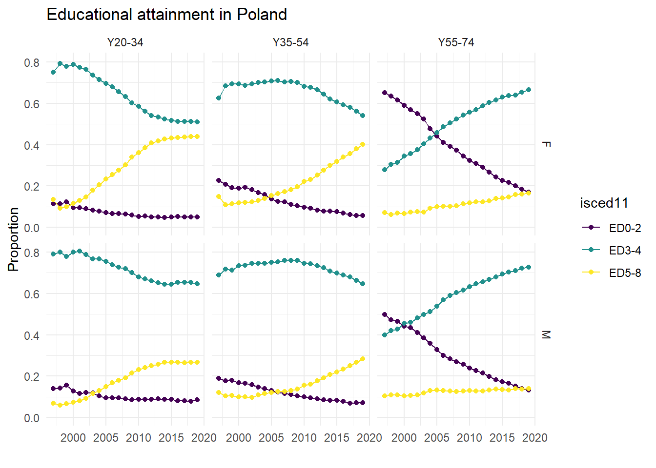
Since within each age and gender combination the proportions in education groups sum to one, it may be better to plot them as a stacked area chart.
edu %>%
  filter(geo == "PL") %>%
  ggplot(., aes(x = time, y = prop_cat, fill = isced11)) +
  geom_area() +
  expand_limits(y = 0) +
  scale_fill_viridis_d() +
  xlab("") +
  ylab("Proportion") +
  ggtitle("Educational attainment in Poland") +
  theme_minimal() +
  facet_grid(sex ~ age_cat)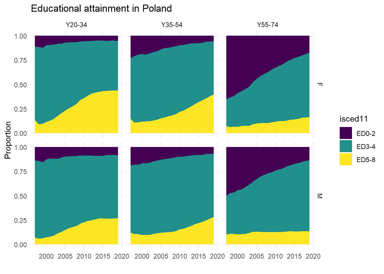
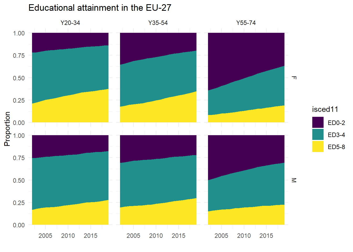
Each country has its own unique pattern, and an overall picture for the EU-27 is shown in the last plot below.
edu %>%
  filter(geo == "EU27_2020") %>%
  ggplot(., aes(x = time, y = prop_cat, fill = isced11)) +
  geom_area() +
  expand_limits(y = 0) +
  scale_fill_viridis_d() +
  xlab("") +
  ylab("Proportion") +
  ggtitle("Educational attainment in the EU-27") +
  theme_minimal() +
  facet_grid(sex ~ age_cat)