
One of the reasons for the harmonization of personal income in addition to household income was to check if the two correlate highly enough to use household income as a substitute for personal income in analyses where economic status is a control variable. This would be great, because household income variables are available in 1177 surveys out of 1721 analyzed in the Survey Data Recycling dataset (SDR) version 1, while personal income only in 453 surveys. Since 419 national surveys from the SDR dataset have data both for personal and for household income, it’s possible to see how the correlations actually look like.
Household and personal income are not part of the SDR v.1 dataset, but they have been harmonized extra and are compatible with the SDR master file. More information about the income source variables and their harmonization can be found in this post. The code used in this post is available here.
Sample correlations
I start by calculating correlations between personal and household income separately for each sample. These two variables have been transformed in a minimal way compared to the original source variables: non-substantive responses (“don’t know”, “not applicable”, “refused”, etc.) were recoded to missing, and in a few cases coding was reversed so that higher values correspond to more income.
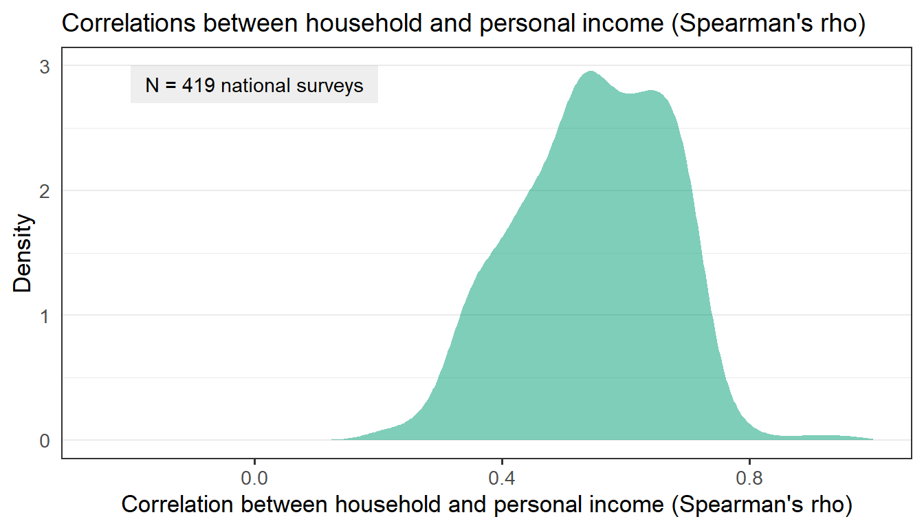
I use Spearman’s rank-order correlation instead of Pearson’s product-moment correlation, because the harmonized income variables have very different distributions in different surveys, as a consequence of the original measurement: in exact income amounts, categories, or quantiles. As shown in the graph below, sample correlations range from 0.2 (ISSP/1991/West Germany) to 0.95 (ISSP/1991/Netherlands), with the mean and median around 0.55.
Sample correlations by gender
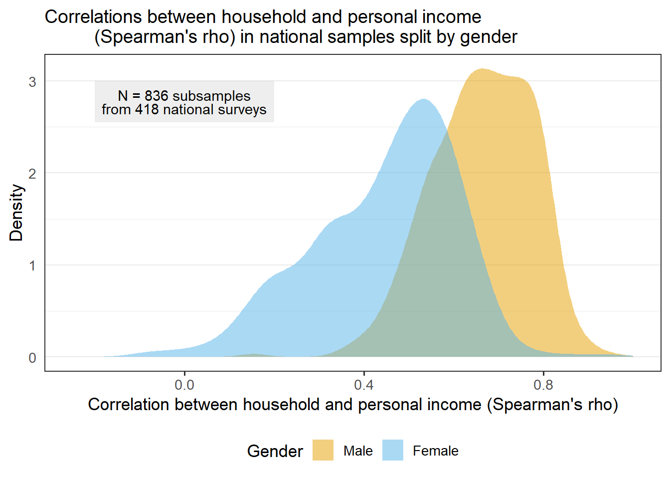
Next I calculate the same correlations separately for the female and male subsamples. The graph below shows that female subsamples account for most of the low correlations. The median correlation for male subsamples is around 0.67, while for female subsamples it’s 0.48. The lowest correlation is -0.088 in the female subsample in ISSP/1991/West Germany, followed by the female subsample in Political Action 2/West Germany (-0.068), ISSP/1989/Netherlands (-0.011) and ISSP/1991/West Germany (-0.006).
Sample correlations by age
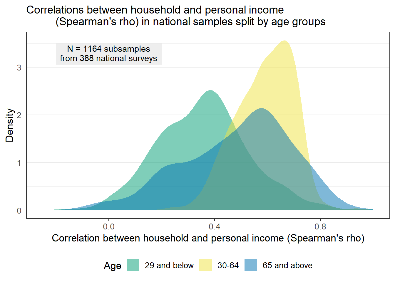
Correlations between personal and household income also vary by age. As shown on the next graph they are lowest among respondents under 30 years of age (median 0.36), followed by those 65 and above (median 0.53), and highest among those aged 30-64 (median 0.6). Because some surveys have only few respondents above 60 years of age, I restrict the analysis to samples where each age group has at least 50 respondents, which is true for 396 national samples.
Sample correlations by education
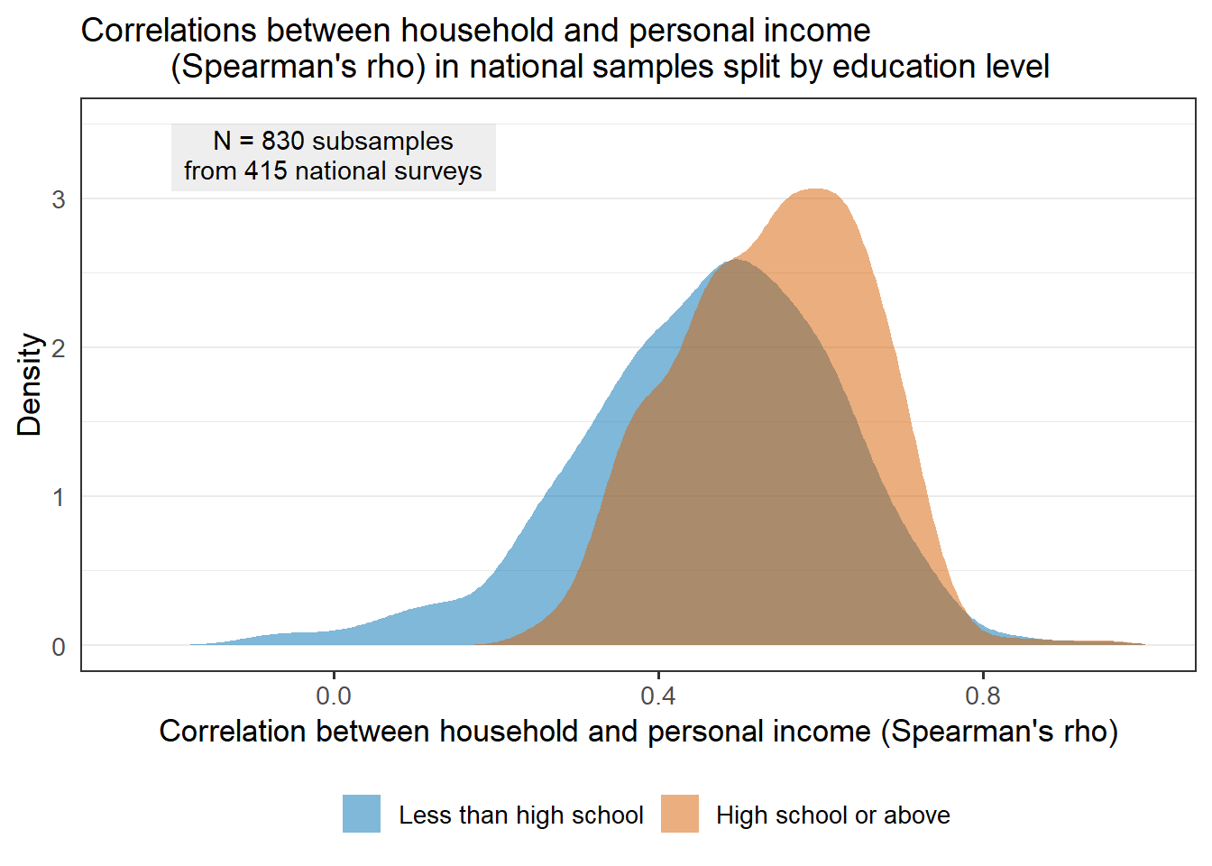
The last examined dimension is education. Correlations between personal and household income are generally higher among those with a high school degree or above (median 0.55) than those with less than high school education (median 0.47).
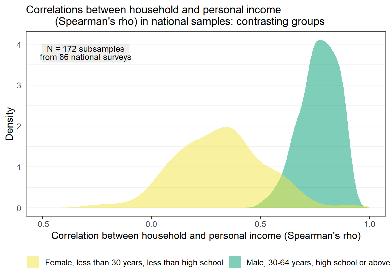
Contrast
I end with a contrast of distributions of correlations between personal and household income for two groups: (1) females, aged less than 30 without high school education (yellow in the graph below), and (2) males, aged 30-64, with high school education or above. Again, I only use surveys that have at least 50 respondents in each of the two groups. In this case it’s just 86 surveys, primarily from the International Social Survey Programme, but also from the from Arab Barometer, the International Social Justice Project, the New Baltics Barometer, and the classic studies from the 1960s and 1970s: Political Action II, Political Action: An Eight Nation Study, and Political Participation and Equality in Seven Nations.
Conclusion
One might say, no wonder the correlations between the two contrasting groups in the last graph are so different when looking at surveys from the 1960s and from Arab countries where a lot of women don’t have their own income. It also makes sense that the correlation is lower for young people, who are more likely to live with parents, and for seniors, who might be living with adult children. The differences between education groups are more difficult to explain and might have to do with larger household size; these differences are also much smaller. All these differences can be investigated. For now the conclusion still is that it’s not realistic to assume that these correlations are universally high or that household income is a universally solid substitute for personal income.